6. The hydrogen atom
Before the advent of quantum theory, it was a mystery why a hydrogen atom (a combination of a negatively charged electron and a positively charged proton), or any other atom, could be stable. Based on classical electromagnetic theory, it was expected that the electron would spiral towards the proton, and the atom would collapse. However, this is contrary to evidence.
The first attempt to rationalize this curious stability of the H atom came from Niels Bohr, who postulated that electrons orbit around protons in circular orbits with the electron having only certain allowed values of angular momentum. This Bohr model imposed stability ad hoc, but it reproduced the position of the lines in the absorption and emission spectra of atomic hydrogen. However, it failed for any atom beyond H. Quantum theory rendered the Bohr model obsolete by not only explaining the H atom, but all other atoms as well. Quantum theory also shows that it is incorrect of thinking of an electron orbiting in a circular orbit around the nucleus - this is a left-over picture from the obsolete Bohr model.
In this chapter, we develop the quantum theory of the hydrogen atom, looking at the energies of its stationary states, the associated wavefunctions, and at the possible transitions between the states.
6.1. Central potential
A hydrogen atom consists of an electron and a nucleus (proton). It is a special case of a one-electron atom (a so-called hydrogenic atom) consisting of one electron and a nucleus with charge number \(Z\): \(Z=1\) for H, 2 for He+, 3 for Li2+, etc. Besides H, the latter ions don’t have much chemical relevance, but it is instructive to examine how quantum predictions (wavefunctions and energuies) depend on nuclear charge.
The negatively charged electron and the positively charged nucleus attract each other electrostatically. This attractive Coulomb force is a result of the electrostatic potential energy, or potential for short,
where \(r\) is the distance between the electron and the nucleus. \(e\) is the elementary charge, and the prefactor \(1/4\pi\epsilon_0\) with the electric constant \(\epsilon_0\) makes sure that we stay within the SI system of units and get \(V\) in units of joule. Notice that the potential energy is negative and depends on the inverse distance - the closer the electron to the proton, the lower (more negative) the potential energy. As the distance between the electron and the nucleus increases, the potential energy approaches zero. Figure 6.1 illustrates this potential-energy function.
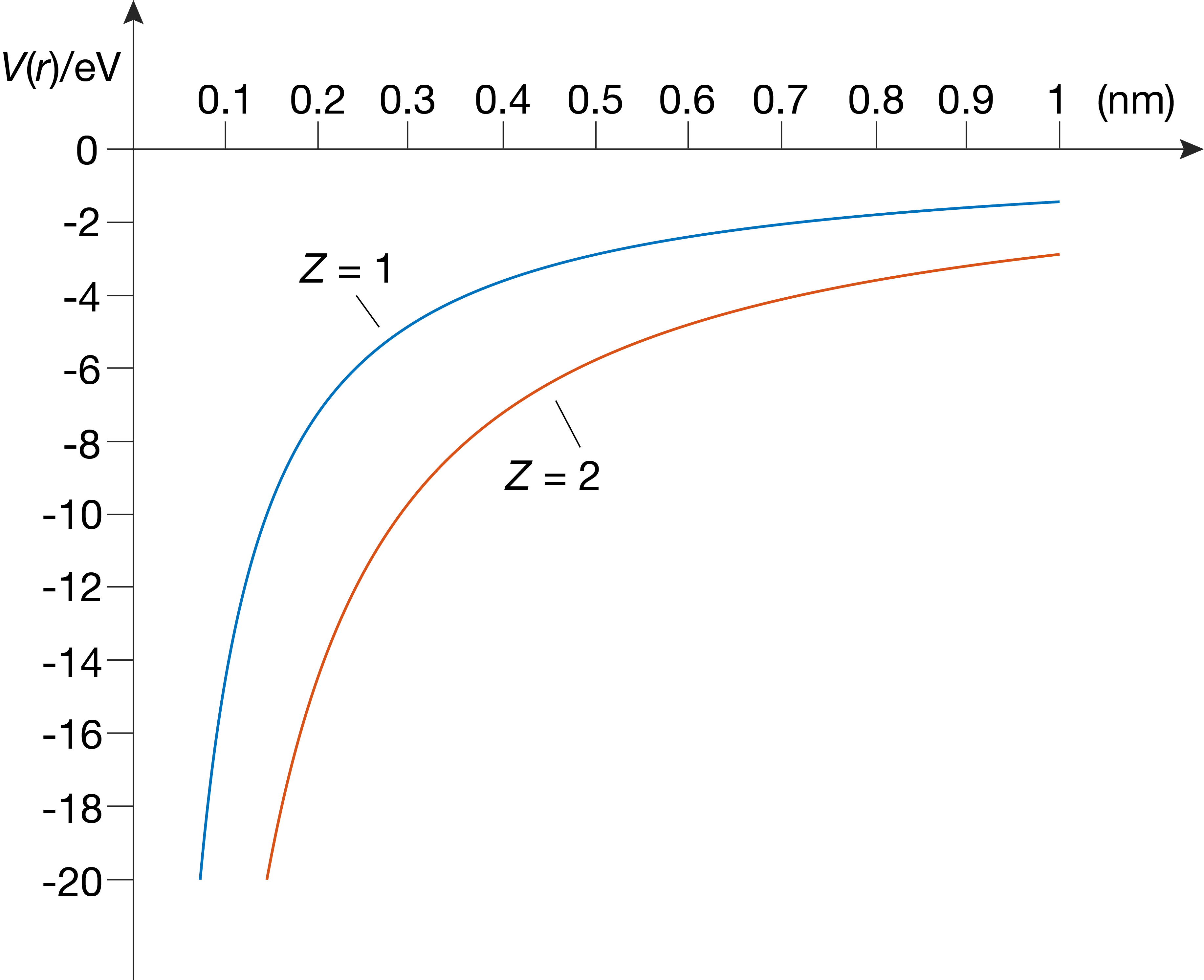
Figure 6.1 The radial electrostatic potential-energy function on the hydrogen atom H (Z = 1) and the helium ion He+ (Z = 2).
Note
It is useful to be aware of the order of magnitude of the electrostatic energy. For an electron that is localized 1.0 Å from a proton, the electrostatic potential energy is about -14 eV.
It is reasonable to consider the proton fixed and the electron moving (just like we consider the sun fixed and the earth moving). This way, the proton constitutes a center that generates a spherically symmetric electrostatic potential in which the electron moves. This is the reason \(V(r)\) is called a central potential.
6.2. The Hamiltonian
With the central potential, the Hamiltonian for a one-electron atom is
For increased accuracy, we should be using the reduced mass of the electron-proton system, \(\mu = m_\mathrm{e}m_\mathrm{p}/(m_\mathrm{e}+m_\mathrm{p})\), however, since the proton (and any other nucleus) has a much larger mass than the electron, we approximate \(\mu = m_\mathrm{e}/(m_\mathrm{e}/m_\mathrm{p}+1)\approx m_\mathrm{e}\).
Since we have a spherically symmetric situation, it is mathematically most convenient to use spherical coordinates \(r\), \(\theta\), and \(\phi\). The wavefunction is a function of these three coordinates: \(\psi(r,\theta,\phi)\).
As shown in the Appendix, the Schrödinger equation with the above Hamitonian, \(\hat{H}\psi(r,\theta,\phi) = E\cdot\psi(r,\theta,\phi)\) can be solved by separation of variables, writing the wavefunction as a product of three functions, one for each degree of freedom:
with the radial function \(R(r)\) and the angular function \(Y(\theta,\phi)\). We have met the latter before when describing rotations - these are the spherical harmonics. With this, the overall equation can be separated into three equations, one for each degree of freedom. The resulting general mathematical solutions are not all physical - some are not square-integrable. The physical wavefunctions are products
and depend on three integer quantum numbers:
\(n\), the principal quantum number, with possible values 1, 2, etc.
\(l\), the orbital angular momentum quantum number, with possible values 0, 1, …, \(n-1\), and
\(m_l\), the orbital magnetic or orbital projection quantum number, with possible values 0, \(\pm 1\), …, \(\pm l\).
In chemistry, one-electron wavefunction are generally referred to as orbitals, in reference to the orbits of the early Bohr model. In contrast to orbits, in which an electron orbits around the nucleus with fixed \(r\), orbitals capture the fact that the electron is delocalized, i.e. there is a distribution of \(r\)values. An orbital in an atom (like hydrogen) is called an atomic orbital, and an orbital in a molecule (as discussed in the next chapter) is called a molecular orbital.
Depending on the value of the quantum number \(l\), they are indicated with single-letter labels, as given in the following table.
\(l\) |
0 |
1 |
2 |
3 |
4 |
|---|---|---|---|---|---|
letter |
s |
p |
d |
f |
g |
These letter labels are historical and originate in early spectroscopic observations of atomic emissions: s = sharp, p = principal, d = diffuse, f = fundamental. For higher \(l\), the lettering continues alphabetically.
A state with quantum numbers \((n,l,m_l)\) is indicated by \(n\)letter\(_{m_l}\), where \(m_l\) is omitted for s orbitals. The next table lists all states up to \(n=3\).
\(n\) |
\(l\) |
\(m_l\) |
designation |
|---|---|---|---|
1 |
0 |
0 |
1s |
2 |
0 |
0 |
2s |
2 |
1 |
\(-1,0,+1\) |
2p-1, 2p0, 2p+1 |
3 |
0 |
0 |
3s |
3 |
1 |
\(-1,0,+1\) |
3p-1, 3p0, 3p+1 |
3 |
2 |
\(-2,-1,0,+1,+2\) |
3d-2, 3d-1, 3d0, 3d+1, 3d+2 |
Note
The statement “the electron is in the 3s orbital” means “the electron is in the state characterized by the quantum numbers \((n,l,m_l)=(3,0,0)\)”. The associated wavefunction is \(\psi_{3,0,0}(r,\theta,\phi)\).
All states with the same \(n\) are called a shell. Often, particularly in X-ray spectroscopy, these shells are referred to by letters: The shells corresponding to \(n=1,2,3,4,\cdots\) are labeled as K, L, M, N, etc. For example, the L shell comprises the orbitals 2s, 2p-1, 2p0, and 2p+1. Within a shell with a given \(n\), all states with the same \(l\) are called a subshell. The L shell consists of a 2s subshell and a 2p subshell.
6.3. Energy levels
The energies associated with the above wavefunctions are
Note that the expression above contains the inverse square of \(n\), the square of the prefactor of the electrostatic interaction, and the inverse of the prefactor from the kinetic-energy operator in the Hamiltonian.
Note
The important aspects of the energy expression for the bound states are
The energies are quantized, with the quantum number \(n\).
All energies are negative.
They converge to zero as \(n\) increases.
The spacing between the energy levels shrinks with increasing \(n\).
The kinetic energy of the ground state (\(n=1\)) is non-zero, indicating that there is zero-point energy.
Each stationary state in a hydrogenic atom is identified by three quantum numbers (\(n\), \(l\), and \(m_l\)), but the energy depends only on one of them. All the states with the same \(n\) are therefore degenerate. For a given \(n\), there are a total of \(n^2\) degenerate state with the same energy \(E_n\). For example, for \(n=2\), there are \(n^2\) degenerate states: 2s, 2p-1, 2p0, 2p+1. Also, all the \(2l+1\) states with the same \(n\) and \(l\) (but different \(m_l\)) are degenerate.
Note
It is crucial to distinguish between the one-electron atom and multi-electron atoms and molecules. The \(n^2\) states with the same \(n\) are degenerate only in a one-electron atom. In multi-electron atoms and molecules, the electrostatic repulsion between the electrons removes this degeneracy, and the orbitals with the same \(n\) have different energies.
As we have seen with three-dimensional potential wells, a high degree of degeneracy is a consequence of high symmetry. Here, the degeneracy is a consequence of the spherical symmetry of the H atom. Lowering the symmetry in any way will reduce the degree of degeneracy.
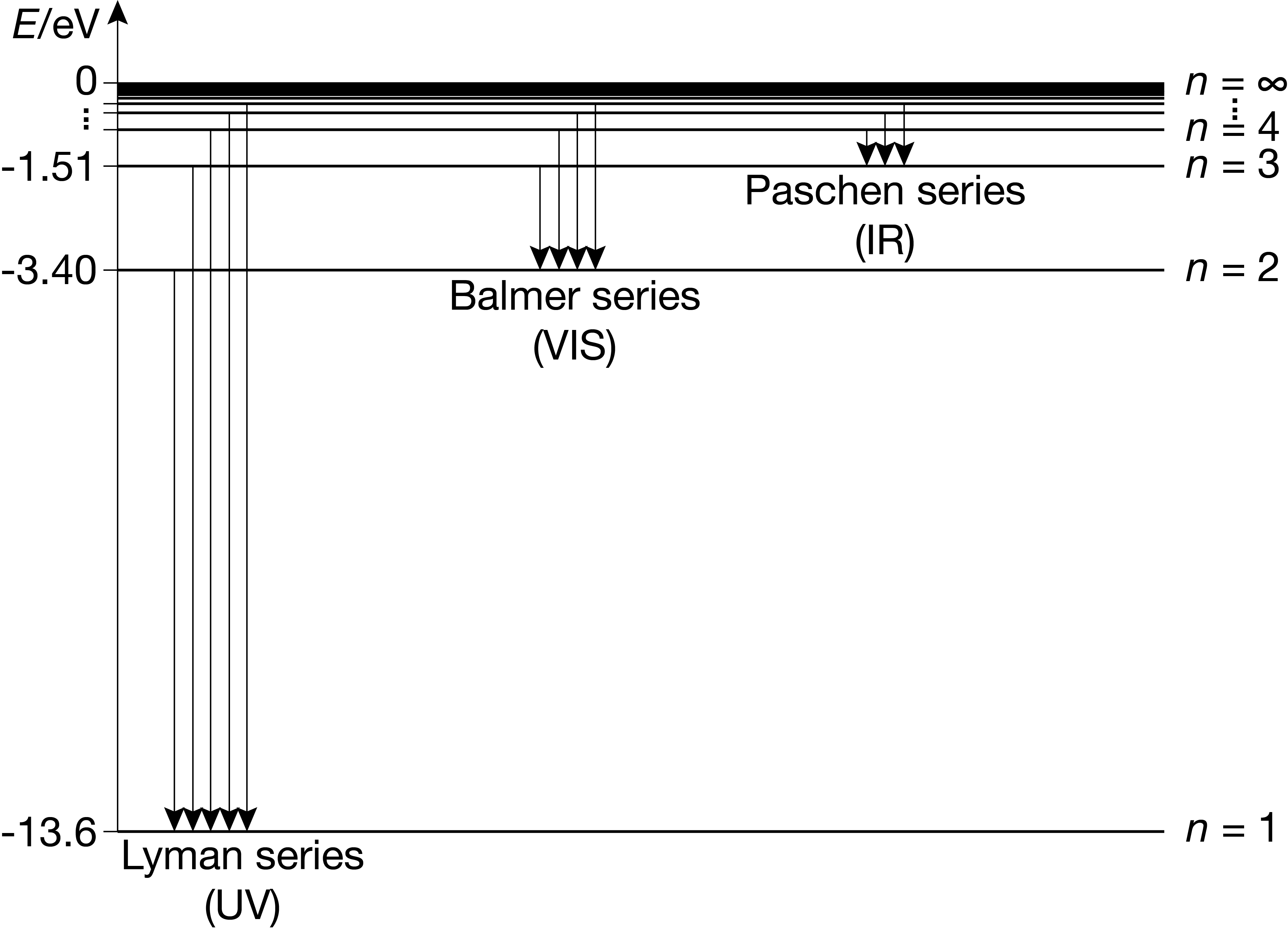
Figure 6.2 The energy levels of the hydrogen atom, and the emission series. Each energy level has \(n^2\) degenerate states.
Figure 6.2 shows the energy level diagram of the hydrogen atom. It also shows the allowed emissive transitions, which we discuss in the next section.
6.4. Emission and absorption spectra
The intensity of an absorption or emission transition between two states with quantum numbers \((n,l,m_l)\) and \((n',l',m'_l)\) is proportional to the electric transition dipole moment:
Mathematically, this integral can be non-zero only if the following selection rules are all satisfied simultaneously:
In addition, of course, for absorption and stimulated emission, the photon energy of the incoming radiation has to match the energy difference of the two states, i.e. \(h\nu = |E_{n'} - E_n|\).
Figure 6.2 illustrates the \(\Delta n\) part of the selection rules: There are no restrictions on how much \(n\) can change in a transition. All emissive transitions with the same target \(n\) are called a series. They are labelled in the figure.
Figure 6.3 shows a slightly more detailed energy level diagram that spreads out groups of states with different \(l\) horizontally. This is called a Grotrian diagram. In this visualization, the selection rule for \(\Delta l\) becomes more evident. For example, vertical transitions (\(\Delta l=0\)) are forbidden.
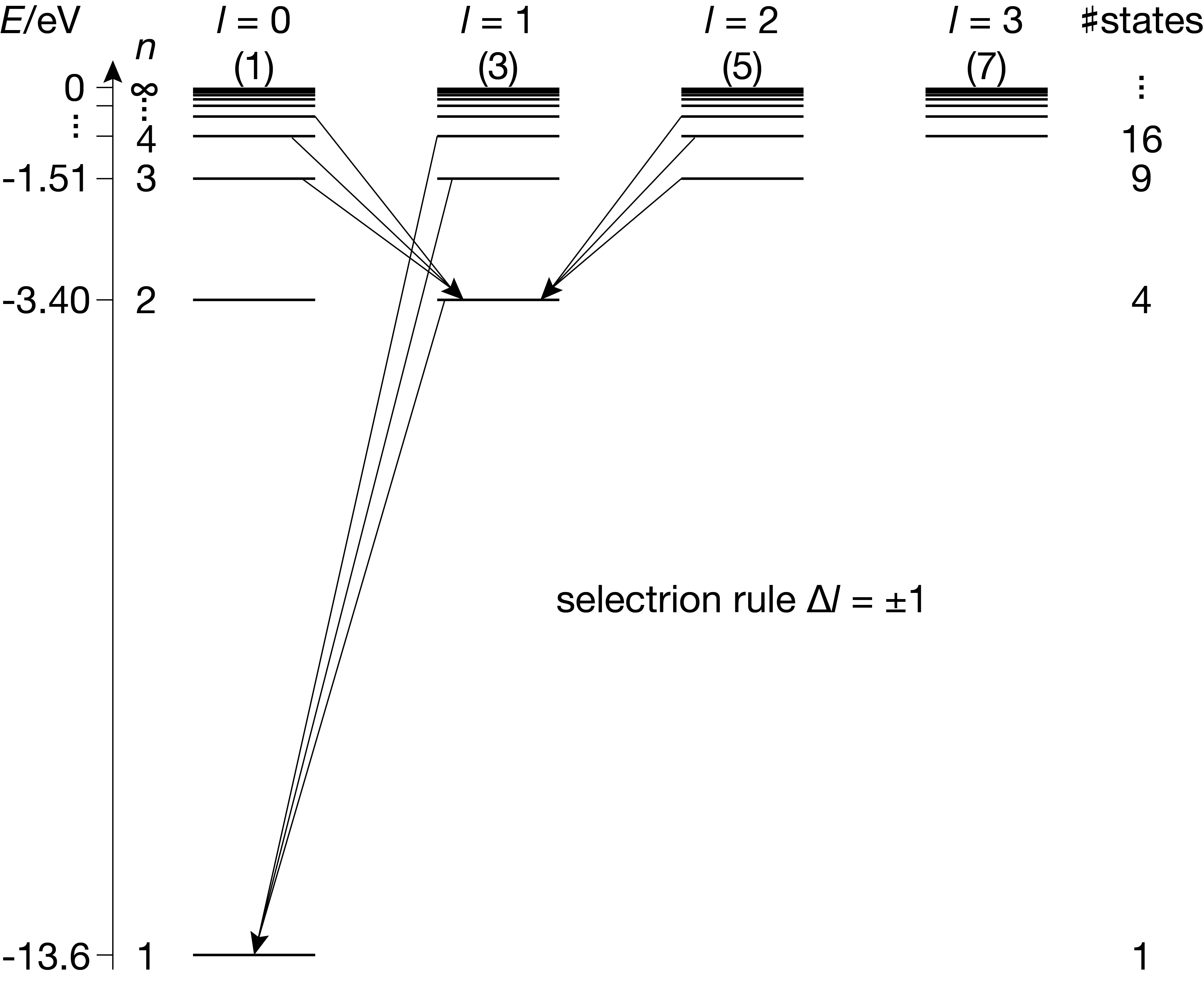
Figure 6.3 Grotrian diagram of the states in the hydrogen atom, with a few of the allowed transitions indicated.
Figure 6.4 shows a schematic emission spectrum of hydrogen. Notice that differnt lines have vastly different intensities: the larger \(\Delta n\), the smaller the intensity. This is a direct manifestation of the different transition dipole moments associated with these transitions.
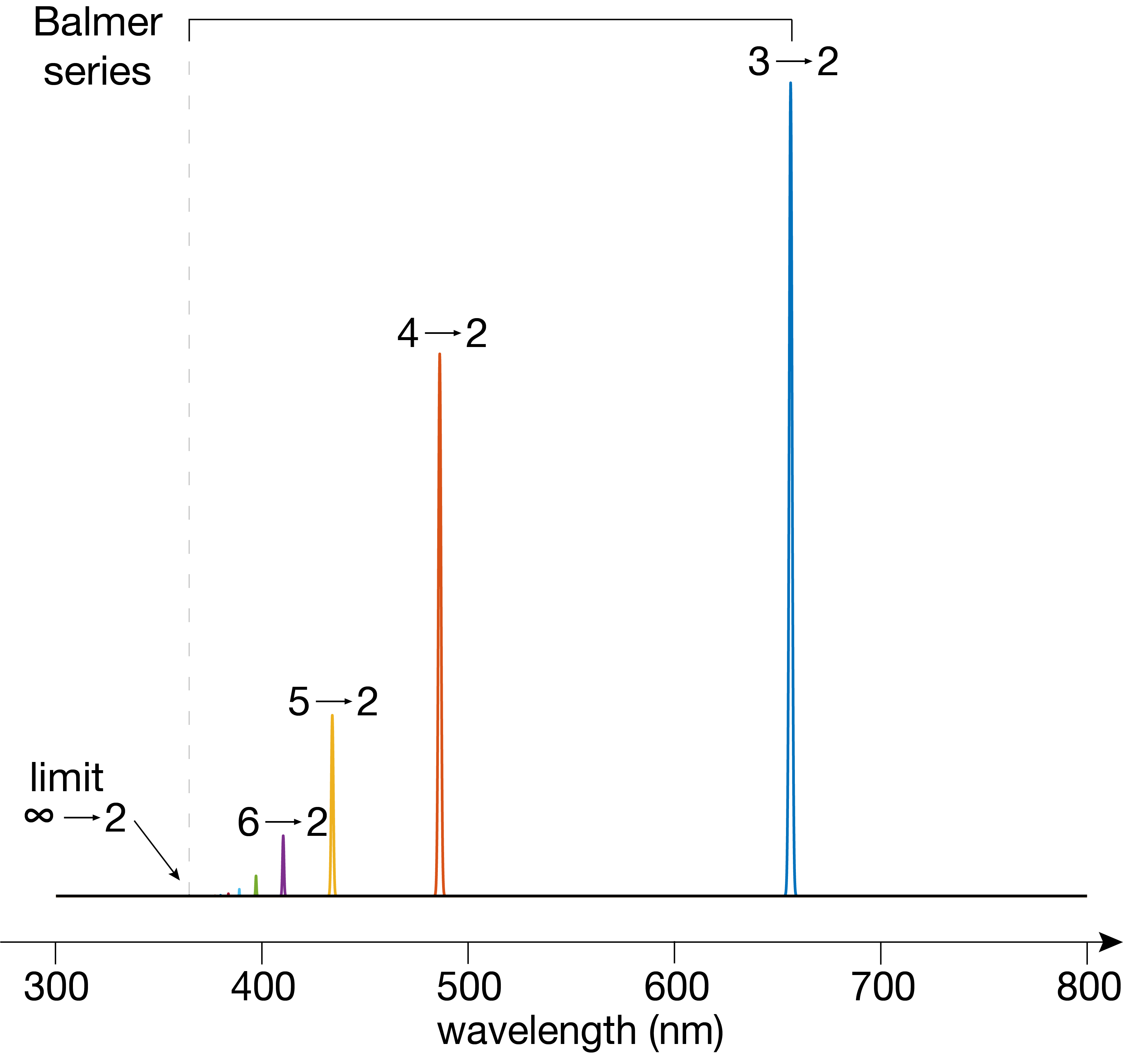
Figure 6.4 The visible part of the emission spectrum of hydrogen atoms. The numbers indicate the quantum numbers \(n\) of the initial and final state involved in each transition.
6.5. Wavefunctions
The wavefunctions for the energy eigenstates of a hydrogenic atom are products of three functions, one for each degree of freedom (\(r\),\(\theta\), and \(\phi\)):
where \(R_{n,l}\) is the radial function, and the spherical harmonic \(Y_l^m\) is the angular function. Each of the functions is normalized by itself, so that the overall wavefunction is normalized as well.
Radial functions. The radial function depends on the quantum numbers \(n\) and \(l\) and is best written in terms of the scaled radius \(\rho = (2Z/n)(r/a_0)\), a unitless quantity:
Here, \(N_{n,l}\) is the normalization constant (which we don’t write out here), and \(L\) is a so-called associated Laguerre polynomial. For a derivation of the radial functions, see the appendix.
Here is a brief table of some of the radial functions up to \(n=3\):
Symbol |
\(n\) |
\(l\) |
\(R_{n,l}\) |
|---|---|---|---|
1s |
1 |
0 |
\(R_{1,0}\propto \mathrm{e}^{-\rho/2}\) |
2s |
2 |
0 |
\(R_{2,0}\propto (2-\rho)\cdot\mathrm{e}^{-\rho/2}\) |
2p |
2 |
1 |
\(R_{2,1}\propto \rho\cdot\mathrm{e}^{-\rho/2}\) |
3s |
3 |
0 |
\(R_{3,0}\propto (6-6\rho+\rho^2)\cdot\mathrm{e}^{-\rho/2}\) |
3p |
3 |
1 |
\(R_{3,1}\propto (4\rho-\rho^2)\cdot\mathrm{e}^{-\rho/2}\) |
3d |
3 |
2 |
\(R_{3,2}\propto \rho^2\cdot\mathrm{e}^{-\rho/2}\) |
Figure 6.5 illustrates these functions. They have the following features: (1) They are oscillatory and decay exponentially as \(r\rightarrow\infty\). (2) They are independent of the angles. (3a) They have \(n-l\) lobes (half “waves”). So s orbitals have \(n\) lobes, p orbitals have \(n-1\) lobes, and so on. (3b) They have \(n-l-1\) nodes, not counting \(r=0\). So s orbitals have \(n-1\) nodes, p orbitals have \(n-2\) nodes, etc. (4) Only s orbitals (\(l=0\)) are non-zero at \(r=0\), the position of the nucleus.
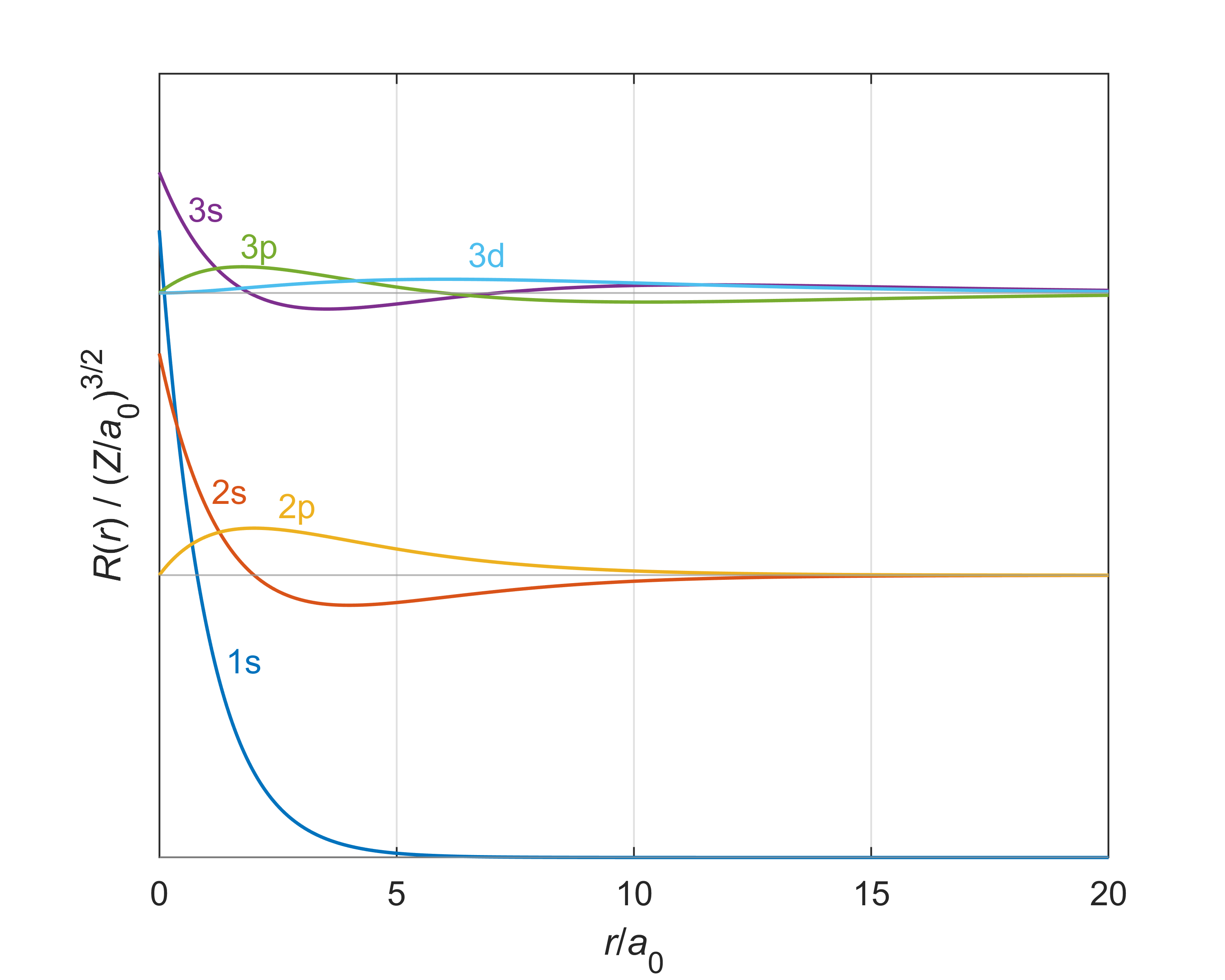
Figure 6.5 The radial functions \(R_{n,l}(r)\) of the hydrogen atom for \(n = 1\), \(2\), and \(3\).
The radial functions are normalized, satisfying the normalization condition
The \(r^2\) factor in the integral is the radial part of the volume element in spherical coordinates.
The integrand in the above integral is called the radial probability density and gives the probability density of finding the electron in a region \(\mathrm{d}r\) around a distance \(r\) from the nucleus no matter what the orientation. Figure 6.5 illustrates this quantity.
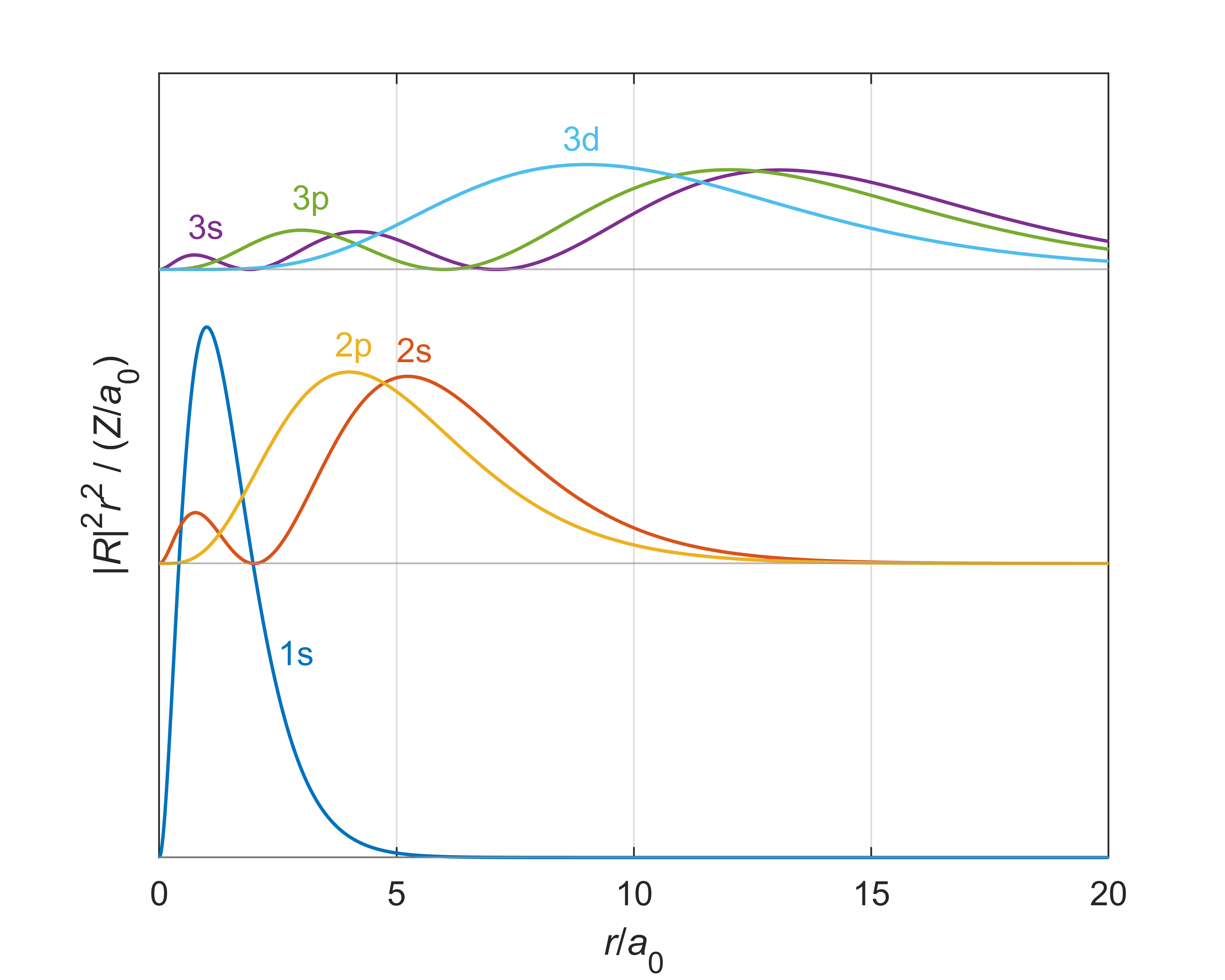
Figure 6.6 The radial probability densities \(|R_{n,l}|^2r^2\) for all states with \(n\) up to 3.
With this, one can calculate the total probability of finding the electron in a radial range from \(r_\mathrm{min}\) to \(r_\mathrm{max}\)
Angular functions. The angular functions are the spherical harmonics, which we already encountered in the context of the rigid rotor:
where \(N_{l,m}\) is again a normalization factor, and \(P_{l,|m|}(\cos\theta)\) is the associated Legendre polynomial. The normalization is such that
Expectation values. To calculate the expectation value of any observable for a hydrogenic wavefunction, we have to integrate over all space in spherical coordinates:
Note
The expectation value of the radius, \(\langle r\rangle\), for the hydrogen atom in the ground state is
where \(\psi_\mathrm{1s} = (1/\pi a_0^3)^{1/2}\mathrm{exp}(-r/a_0)\) is the ground-state wavefunction. This 3D integral can be factored into three separate integrals, and since \(\psi_\mathrm{1s}\) only depends on \(r\), it ends up in the \(r\) integral:
The \(\theta\) integral evaluates to 2, the \(\phi\) integral to \(2\pi\), and the radial integral is
so that the final result is
This means that “on average” one will find the electron \(3a_0/2\) away from the nucleus.
Real-valued orbitals. All the states with the same \(l\), but different \(m_l\) are degenerate, so any linear combination of them also has the same energy. We can use this property to construct real-valued wavefunctions. The wavefunctions with \(m_l=0\) are already real-valued, but those with \(m_l\neq0\) are complex-valued due to the presence of the factor \(\mathrm{exp}(\mathrm{i}m_l\phi)\). The wavefunction with identical \(n\) and \(l\) and with \(m_l\) of opposite sign can be linearly combined into a real-valued wavefunction, based on the following relationships
Note
For example, the real-valued \(p_x\) and \(p_y\) wavefunctions are the cos and sin combination of \(p_{-1}\) and \(p_{+1}\):
For the \(d\) orbitals, the real-valued combinations are
6.6. Conceptual aspects
Location of electron. One important conceptual question is: “Where is the electron really?”. Quantum theory’s answer is somewhat disappointing: “We don’t know, but quantum theory predicts that, if we take a hydrogen atom in the \((n,l,m_l)\) state and measure the electron position, we will find it with probability
in an infinitesimal volume around the point \((r,\theta,\phi)\)“.
Instead of giving a precise circular orbit (like in popular perception, and in the pre-quantum Bohr model), quantum theory only provides statistical predictions about the whereabouts of the electron. Unfortunately, this is the current state of our experimental capabilities and our predictive theory.
This illustrates once again that quantum theory is a statistical theory that makes purely probabilistic predictions about the outcomes of tests or measurements. In that sense, it is like sports statistics: Even knowing all the data and past performance about an athlete or a team, it is impossible to predict with certainy the outcome of the next competition or game. Albert Einstein was dissatisfied by this apparent lack of certainty in quantum theory: “God doesn’t play dice”.
Note
The expression “the electron is delocalized”, which is a core phrase in chemistry, is nothing but a statement that it can be found anywhere in a larger region of space with non-zero probability, in the sense of the above equation. In other words, it is our knowledge about the electron that is fuzzy (delocalized), and not the electron itself.
Stability of H atom. A second question is “Why is the hydrogen atom stable”? Why doesn’t the electron collapse into the nucleus due to the electrostatic attraction? One possible explanation is as follows. Assume a 1s wavefunction with a variable parameter \(a\) in place of the Bohr radius \(a_0\):
By varying \(a\), the wavefunction can be changed: lowering \(a\) below \(a_0\) concentrates it more around the nucleus, and increasing \(a\) above \(a_0\) makes it more delocalized. We can now plot the expectation values of the kinetic energy and of the potential energy, \(\langle T\rangle\) and \(\langle V\rangle\), as well as the total energy \(E\), all as a function of \(a\). If the atom is stable, there should be a minimum in \(E(a)\). This is indeed the case, as illustrated in Figure 6.7.
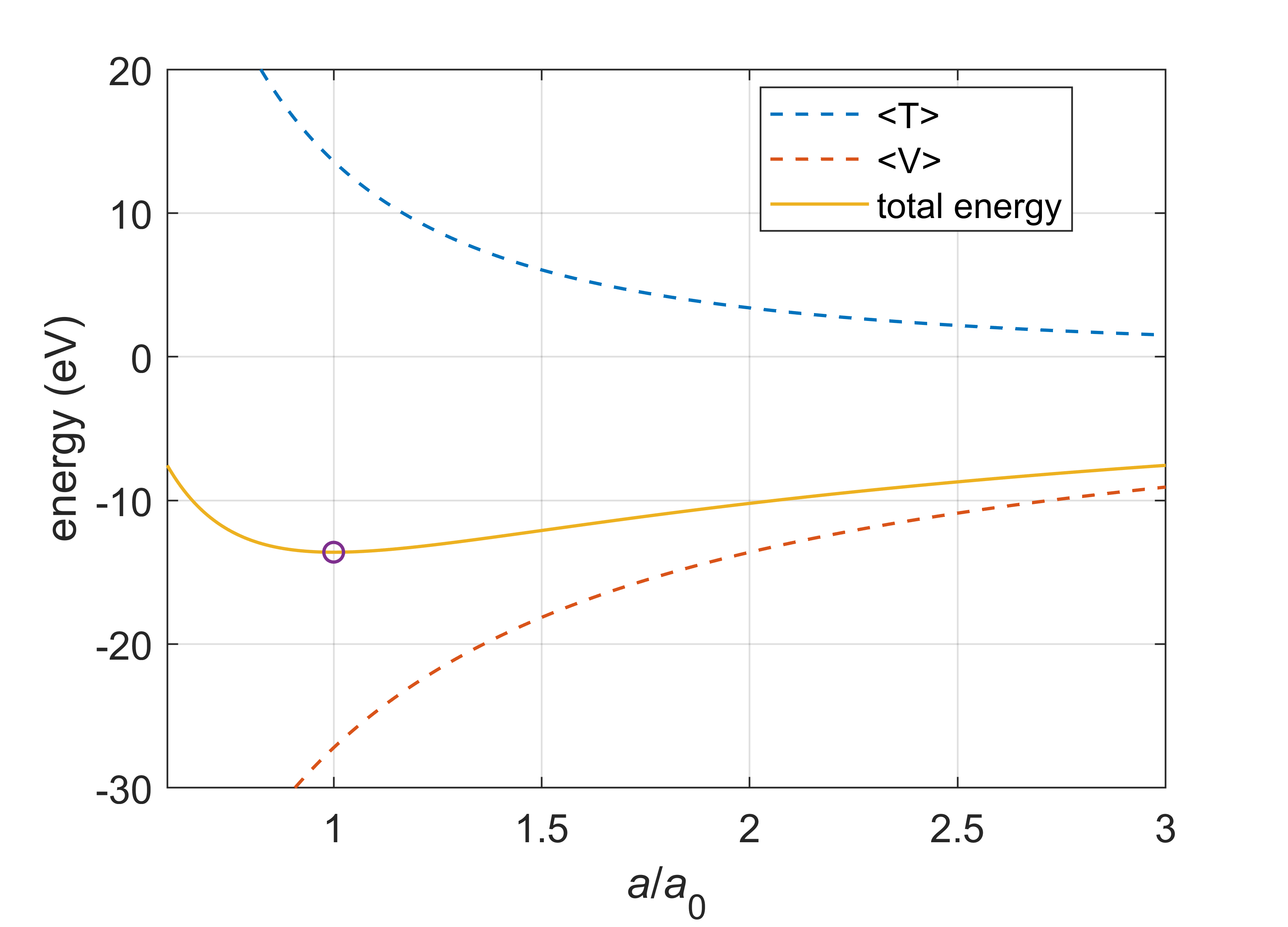
Figure 6.7 Kinetic, potential, and total energy of the adjustable 1s wavefunction \((1/\pi a^3)^{1/2}\mathrm{exp}(-r/a)\), with variable parameter \(a\) instead of \(a_0\). The total energy has a minimum at \(a=a_0\).
With decreasing \(a\), the potential energy becomes more favorable, decreasing with \(1/a\). Based on the potential energy alone, the electron would therefore collapse into the nucleus. However, the kinetic energy grows with \(1/a^2\) as \(a\) decreases. This means that at very short distances the increased kinetic energy outweighs the lowered potential energy. Therefore, there is a minimum. It occurs at \(a=a_0\). The extent of the 1s orbital is a compromise between potential energy and kinetic energy, with the potential energy attracting the electron to the nucleus, and the kinetic energy providing “pressure” that keeps the electron away from the nucleus. Since the kinetic energy is involved, the stability of the hydrogen atom is not a pure electrostatic effect, but a dynamic effect.