5. Molecular rotations

In this chapter, we look at the quantum-theoretical description of rotational motion. This is relevant for modeling molecules tumbling in the gas phase (but not in the liquid or solid state). It will also be important for the describing the angular motion of electrons around a nucleus in an atom, which we will examine in the next chapter.

From the purpose of describing their rotational behavior, molecules fall into several groups based on their overall symmetry: linear rotors, spherical tops, symmetric tops, asymmetric tops. Examples for these four symmetry types are shown in Figure 5.1.

Figure 5.1 Molecules categorized by the symmetry of their moments of inertia. A, B and C indicate three perpendicular axes.

In this chapter, we will only examine the simplest case of rotational motion, that of a linear diatomic molecule. Initially, we will assume that the molecule is a linear rigid rotor, i.e. that it does not vibrate and that its bond length is unaffected by the rotational motion. At the end of the chapter, we will examine how to extend the description to situations where these assumptions are not fully correct.

The rotational behavior of a molecule depends on its moments of inertia around three perpendicular axes (indicated by A, B and C in Figure 5.1).

5.1. Linear rigid rotor

The characteristic property of a diatomic molecule that determines its rotational behavior is its moment of inertia around an axis perpendicular to the bond axis \(A\).

(5.1)\[I_B = I_C = \mu r_\mathrm{e}^2 = I\]

Here, \(\mu\) indicates the reduced mass \(\mu = m_1m_2/(m_1+m_2)\) and \(r_\mathrm{e}\) is the equilibrium bond length. The moment of inertia around the molecular axis (z) is zero, \(I_A = 0\).

A linear molecule has two degrees of freedom: it can rotate around either of two axis that are perpendicular to the molecule. Any rotation changes the orientation of the molecule. This orientation in space is best described in a spherical coordinate system, consisting of two angles \(\theta\) and \(\phi\) (see the Appendix). The angle \(\theta\) is the angle down from the z axis, and \(\phi\) is the angle in xy plane. This is illustrated in Figure 5.2.

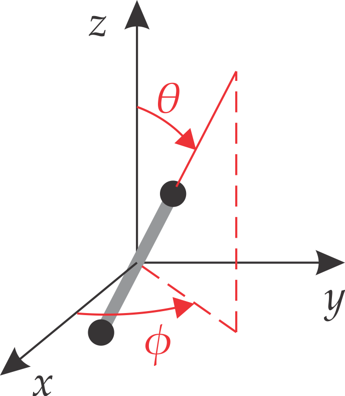
Figure 5.2 Using a spherical coordinate system with angles \(\theta\) and \(\phi\) to describe the orientation of a linear molecule.

Note

Spherical coordinate systems are used many purposes: Locations on earth are specified using a spherical coordinate system with longitude and latitude, where longitude corresponds to \(\phi\), and latitude corresponds to \(\pi/2-\theta\). In astronomy, locations in the sky are also indicated using a spherical coordinate system, and the associated angles are called altitude/elevation and azimuth.

Since we are looking at a rotor that is unconstrainted in its (rotational) motion, its potential energy is independent of orientation and can be set to zero (\(V(\theta,\phi)=0\)). The total energy of the rotor is therefore equal to the kinetic energy. The classical kinetic energy of a rotating body is \(T = \frac{1}{2}I\omega^2 = J^2/2I\), with the angular momentum \(J\) and the angular frequency \(\omega\). To obtain the quantum Hamiltonian from this, we replace \(J\) with its operator \(\hat{J}\):

(5.2)\[\hat{H} = \frac{\hat{J}^2}{2I}\]

Note the analogy to the linear motion, \(\hat{H} = \hat{p}^2/2m\): The angular momentum \(\hat{J}\) takes the place of the linear momentum \(\hat{p}\), and the moment of inertia \(I\) takes the place of the mass \(m\).

With the Hamiltonian in hand, we can set up the Schrödinger equation and solve it. Traditionally, the stationary rotational wavefunctions for a linear rotor are indicated by \(Y\) instead of \(\psi\). The time-independent Schrödinger equation is

(5.3)\[\frac{\hat{J}^2}{2I} Y(\theta,\phi) = E\cdot Y(\theta,\phi)\]

The solution of this equation provides the energies and wavefunctions for the stationary states of the rigid rotor. See the Appendix for the mathematical details. The physical solutions of this equation, \(Y_J^m\), are called spherical harmonics and depend on two quantum numbers \(J\) and \(m\), with possible values \(J = 0,1,\dots\) and \(m = 0,\pm1,\dots,\pm J\). The fact that the quantum number \(m\) must be an integer is a consequence of the requirement that a physically valid wavefunction must be single-valued along \(\phi\), that is, \(Y(\theta,\phi+2\pi)=Y(\theta,\phi)\). The required normalizability along \(\theta\) leads to the requirement that \(J\) must be a non-negative integer, and that \(m\) cannot be larger than \(J\). There are two quantum numbers(\(J\) and \(m\)) since there are two degrees of freedom (\(\theta\) and \(\phi\)).

The energies of the stationary states are

(5.4)\[E_{J,m} = \frac{\hbar^2}{2I}J(J+1) = B J(J+1)\]

Notice that the energies do not depend on the quantum number \(m\). Since there are \(2J+1\) possible values for \(m\) for a given value of \(J\), there are \(2J+1\) degenerate states with the same energy, i.e. the multiplicity is \(2J+1\). \(B\) is called the rotational constant, and is traditionally given as its wavenumber equivalent, \(\tilde{B} = B/hc\), in units of inverse centimeters (cm^-1).

Note

Typical values of \(\tilde B = B/hc\) for diatomic molecules range from 60.8 cm^-1 for H₂ (dihydrogen) to 0.037 cm^-1 for ¹²⁷I₂ (diiodine). The values decrease with increasing mass of the atoms, since the moment of inertia increases. All values are small relative to the thermal energy \(k_\mathrm{B}T\) at room temperature, which corresponds to about \(k_\mathrm{B}T/hc\approx\) 200 cm^-1.

Figure 5.3 shows the rotational energy level diagram. The ground state (\(J=0\), \(m=0\)) is non-degenerate, and its energy is zero, unlike the particle in the box and the harmonic oscillator. This means the molecule is at rest and does not rotate if it is in its rotational ground state. All exited states (\(J>0\), all \(m\)) are degenerate, with the degeneracies increasing with increasing \(J\). Degenerate states have identical \(J\), but different \(m\). The spacing between adjacent sets of degenerate states increases with increasing energy: \(2B\) between \(J=0\) and \(J=1\), \(4B\) between \(J=1\) and \(J=2\), etc.

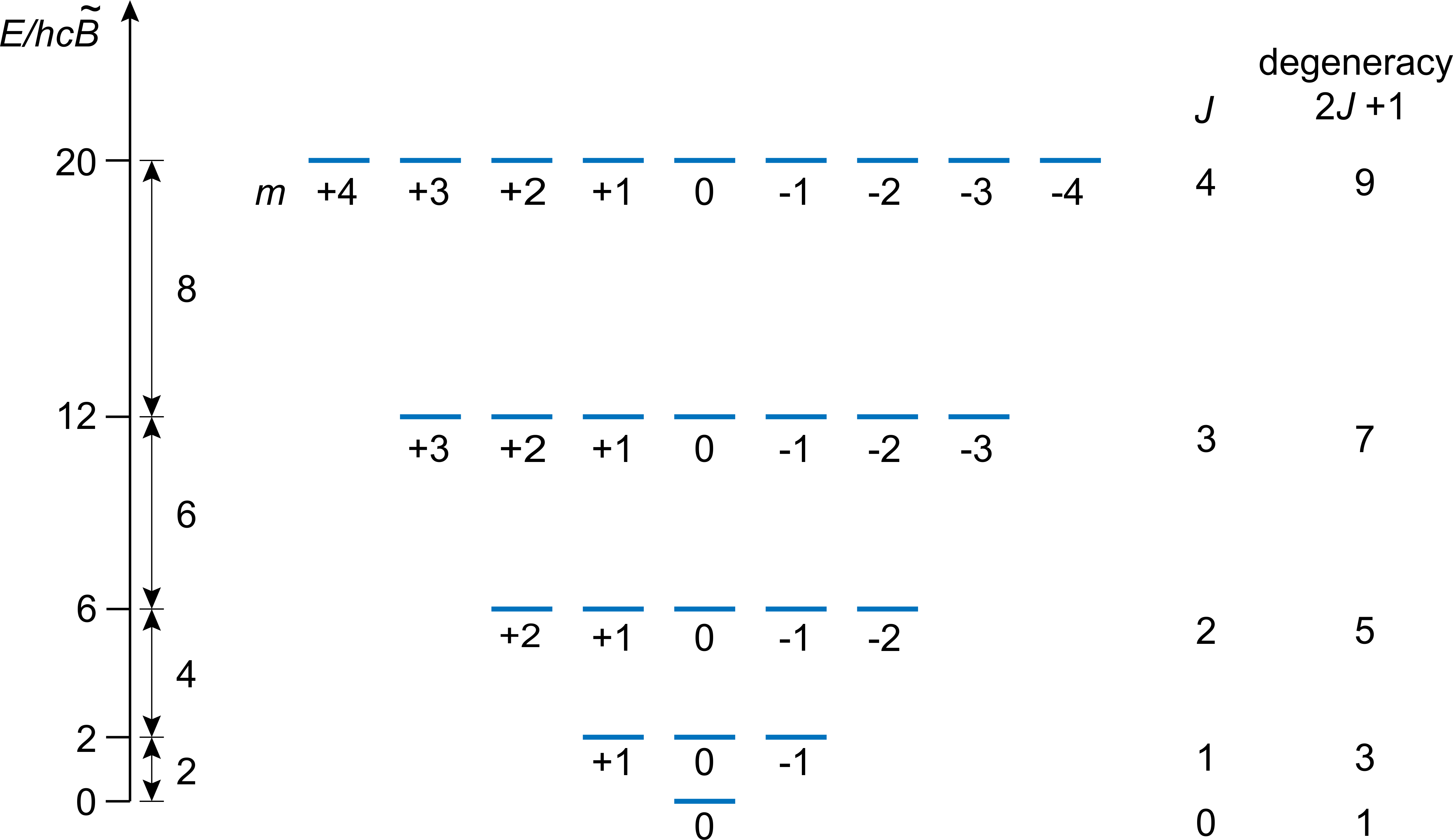
Figure 5.3 Rotational energy levels for a linear rigid rotor, up to \(J=4\).

5.2. Wavefunctions

The eigenfunctions of the rotational Hamiltonian are the spherical harmonics \(Y_J^m(\theta,\phi)\). They are products of a \(\theta\)-dependent function and a \(\phi\)-dependent function

(5.5)\[Y_J^m(\theta,\phi) = N_J^{|m|}\cdot P_J^{|m|}(\cos\theta)\cdot\mathrm{e}^{+\mathrm{i} m\phi}\]

The last factor is a complex-valued exponential. The functions \(P_J^{|m|}\) are special functions called associated Legendre polynomials. Their specific form depends on \(J\) and \(|m|\). \(N_J^{|m|}\) is a real-valued normalization constant such that the wavefunction is normalized:

(5.6)\[\langle Y_J^m|Y_J^m\rangle = \int_0^{2\pi} \int_0^\pi\! |Y_J^m|^2\,\sin\theta \mathrm{d}\theta \mathrm{d}\phi = 1\]

Two spherical harmonics that differ in either \(J\) or \(m\), or both, are orthogonal. Therefore, the spherical harmonics form a complete orthonormal set: \(\langle Y_J^m|Y_{J'}^{m'}\rangle = \delta_{J,J'}\delta_{m,m'}\).

Figure 5.4 illustrates the probability densities \(|Y_J^m(\theta,\phi)|^2\) associated with the stationary states. The wavefunction for the rotational ground state is \(Y_0^0(\theta,\phi) = 1/\sqrt{4\pi}\) and is independent of \(\theta\) and \(\phi\). This gives \(|Y_0^0|^2 = 1/4\pi\) for the probability density, which is independent of the angles. This indicates that the molecule in the rotational ground state is equally likely to be found in any orientation when measured.

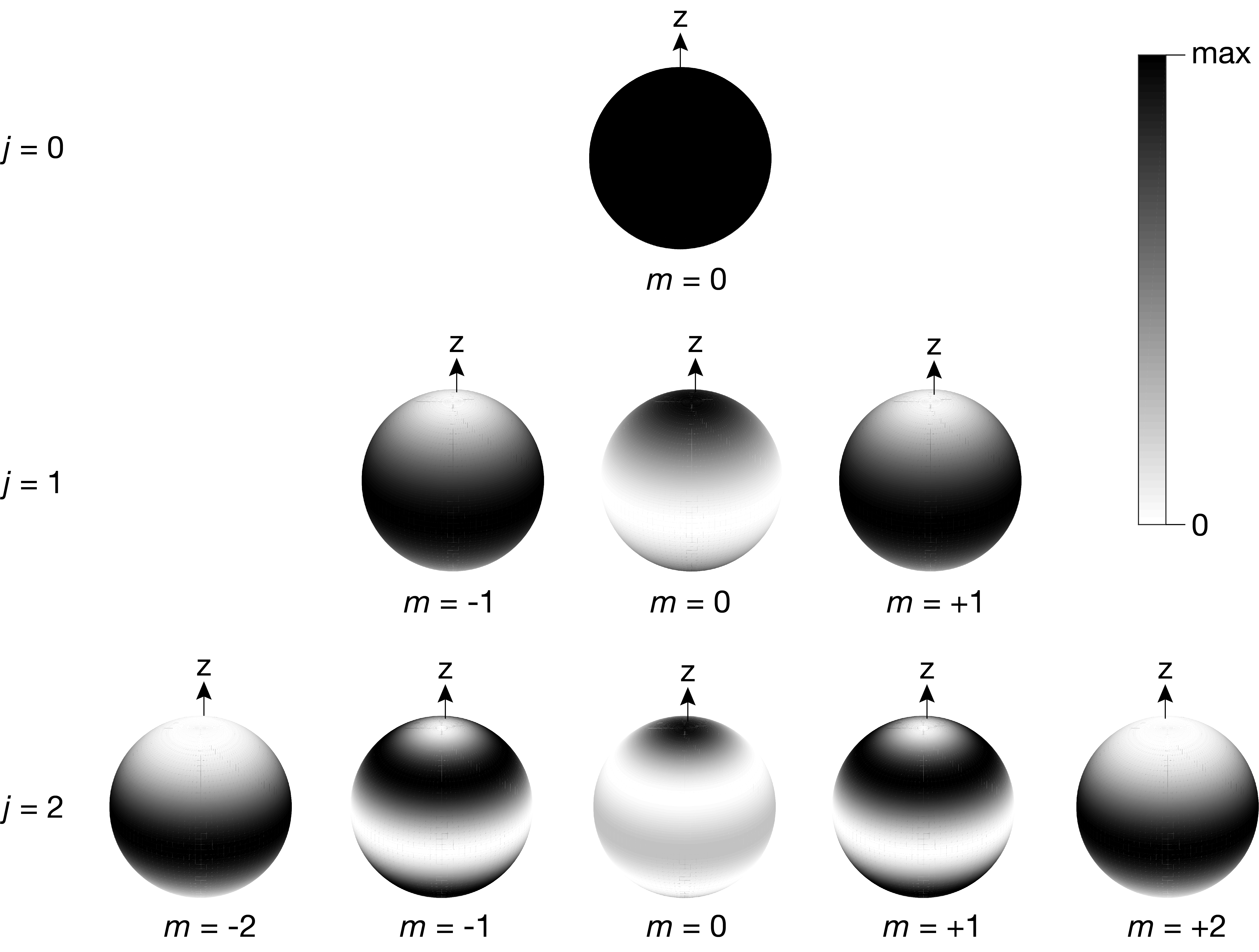
Figure 5.4 Rotational probability densities for some rotational eigenstates. White indicates low, and black indicates high probability density.

The explicit expressions for the wavefunctions of the three states with \(J = 1\) (with \(m = 0\), \(\pm1\)) are

(5.7)\[Y_1^0 = \left(\frac{3}{4}\right)^{1/2}\cos\theta \qquad Y_1^{\pm1} = \mp \left(\frac{3}{8\pi}\right)^{1/2} \sin\theta \cdot \mathrm{e}^{\pm\mathrm{i}\phi}\]

(The overall sign conforms to the Condon-Shortley convention, but is inconsequential here.) Since all states with equal \(J\) have the same energy, any linear combination thereof also has the same energy.

5.3. Rotational spectroscopy

The intensity of a light-induced transition between two rotational states with quantum numbers \(J,m\) and \(J',m'\) is proportional to the transition electric dipole moment squared:

(5.8)\[\mathrm{intensity}\propto |\langle Y_{J'}^{m'}|\hat{\boldsymbol{\mu}}_\mathrm{el}|Y_J^m\rangle|^2\]

The conditions under which this integral is nonzero give the selection rules for rotational transitions: (1) The molecule has to have a permanent electric dipole moment. This means that molecules such as N₂ and H₂ do not undergo rotational transitions, since they don’t have a permanent electric dipole moment. On the other hand, polar molecules like HCl or CO have a permanent electric dipole moment and therefore can undergo rotational transitions. (2) The rotational quantum numbers must satisfy

(5.9)\[\Delta J = J'-J = \pm1\qquad\text{and}\qquad \Delta m = m' - m = 0,\pm1\]

Rotational transitions that satisfy these selection rules are called “allowed”. The energy difference across an allowed rotational transition from \(J\) to \(J+1\) is

(5.10)\[\Delta E_{J+1\leftarrow J} = 2 B (J+1) = 2 h c \tilde{B} (J+1)\]

The incident photon energy must match this energy gap in order for absorption to happen.

Figure 5.5 shows a prototypical rotational absorption spectrum, plotted as a function of the wavenumber of the incident light. The spectral range is in the far infrared and microwave regions of the electromagnetic spectrum (100 cm^-1 corresponds to a wavelength of 100 µm).

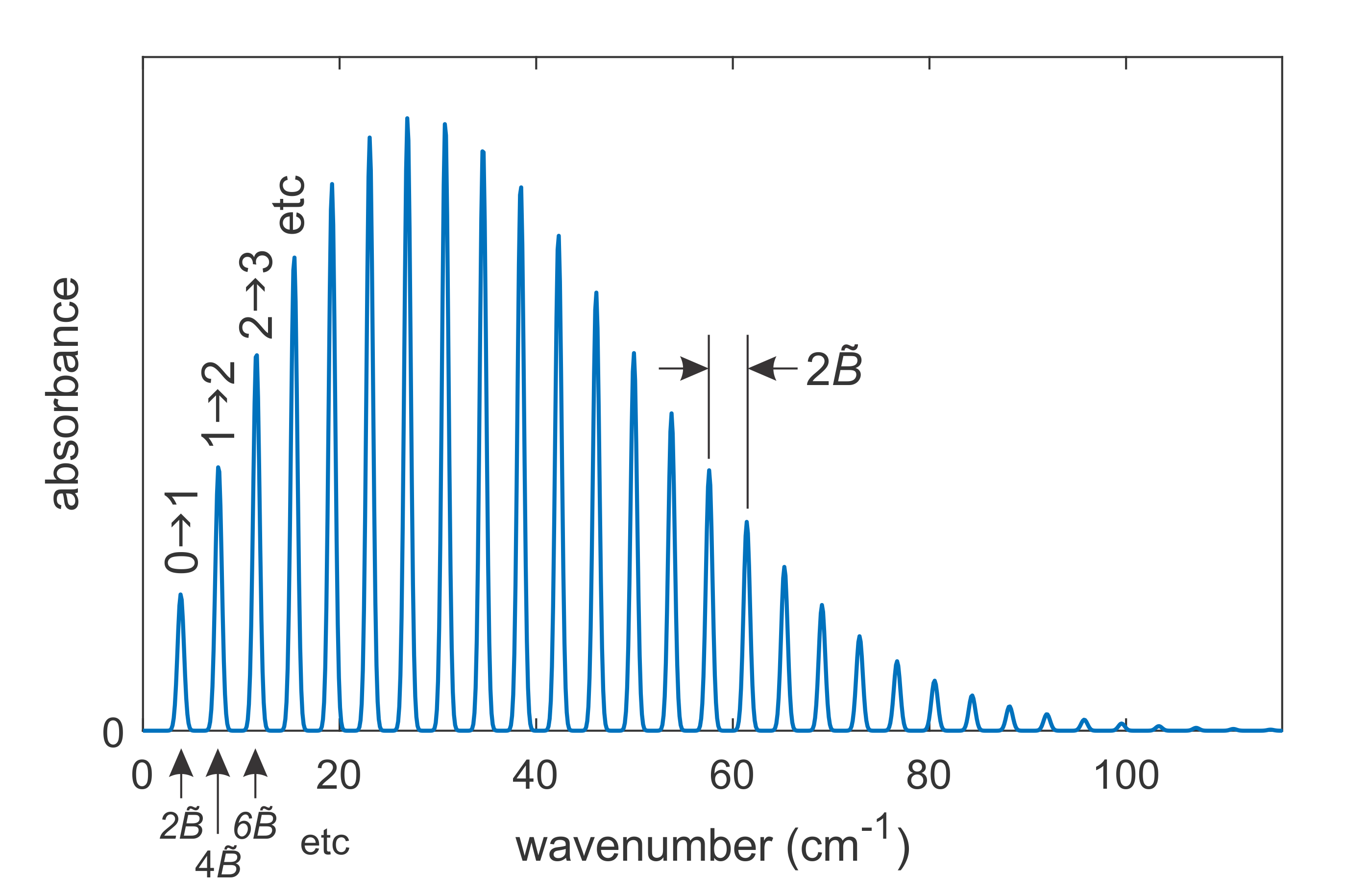
Figure 5.5 Rotational spectrum of a diatomic molecule, here for carbon monoxide ¹²C¹⁶O with \(B/hc\) = 1.9313 cm^-1.

The spectrum consists of a series of equidistantly spaced lines. The spacing between adjacent lines in this spectrum is \(2\tilde{B}\). From this, \(\tilde{B}\) can be extracted. This, in turn, provides information about the moment of inertia \(I\) and the bond length \(r_\mathrm{e}\), since \(hc\tilde{B}=\hbar^2/2I\) and \(I=\mu r_\mathrm{e}^2\). Therefore, gas-phase rotational spectra reveal bond lengths in diatomic molecules with very high accuracy.

Note

Rotational emission spectroscopy is an important remote sensing tool in astronomy. It allows the identification of molecules in interstellar space.

5.4. Rovibrational spectroscopy

In the gas phase, a molecule simultaneously rotates and vibrates. Figure 5.6 shows a schematic energy level diagram of such a molecule. Two manifolds (groups of levels) are shown: the lower manifold is the vibrational ground state (\(n=0\)), and the upper manifold is the first excited vibrational state (\(n=1\)). Each manifold consists of a series of rotational levels with quantum numbers \(J=0, 1, 2, \dots\).

The selection rules for transitions between the two vibrational manifolds are

(5.11)\[n'-n = \pm 1 \qquad \text{and} \qquad J'-J=\pm 1\]

Figure 5.6 shows the two groups of transitions with \((n,J)\leftrightarrow (n+1,J-1)\) (called the P branch) and \((n,J)\leftrightarrow(n+1,J+1)\) (R branch). R-branch transitions are higher in energy than P-branch transitions.

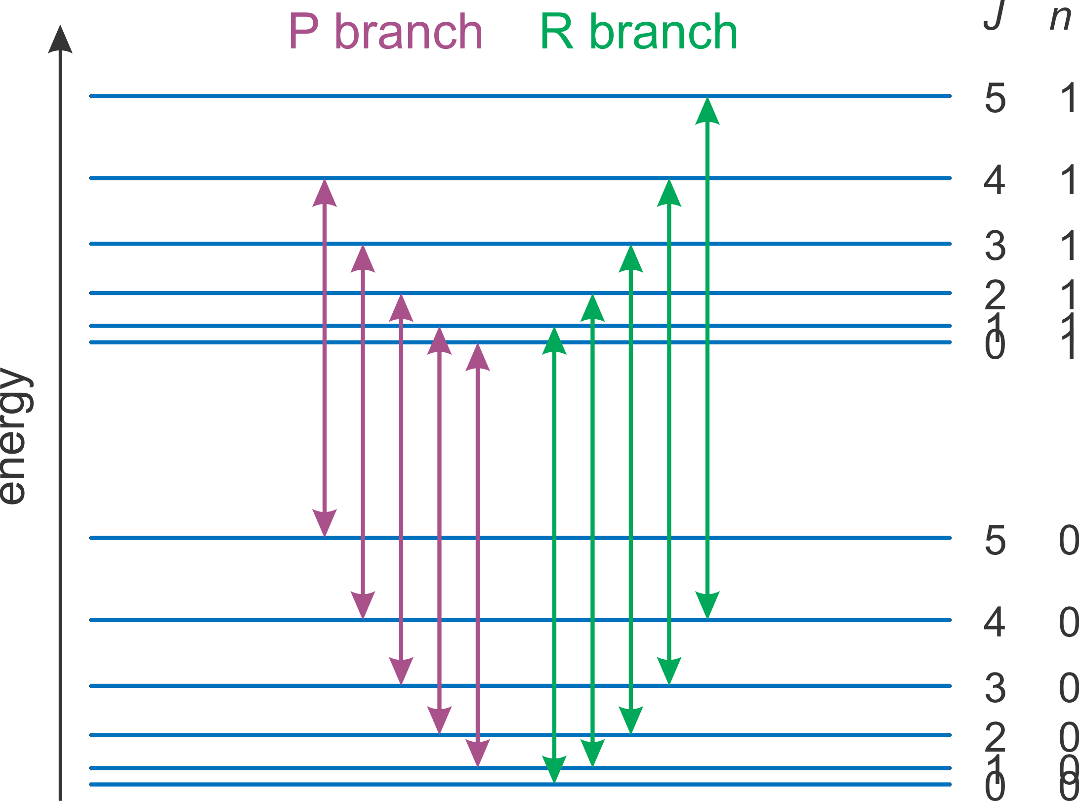
Figure 5.6 Energy level diagram for the two lowest vibrational manifolds (ground state \(n=0\) and first excited state \(n=1\), with rotational sublevels; degenerate states are not shown separately). The purple and green vertical lines indicate the allowed rovibrational transitions.

Figure 5.7 shows an example of a ro-vibrational spectrum (i.e. a vibrational spectrum with rotational fine structure) for a diatomic molecule. Note that there is no absorption at exactly \(\tilde\nu_\mathrm{e}\). This means that light cannot induce a pure vibrational transition from \((n,J)\) to \((n+1,J)\), without an accompanying change in rotational state.

Figure 5.7 Rovibrational spectrum of a diatomic molecule (¹²C¹⁶O at 300 K).

5.5. Non-rigid rotor

Molecules are not rigid. If a molecule rotates, it experiences centrifugal forces, and its bonds stretch. This centrifugal distortion is absent in the rotational ground state (\(J=0\)), but increases with increasing \(J\) (i.e. when the molecule rotates faster). As a consequence, the bond length gets longer, the moment of inertia increases, and the effective \(B\) decreases. To account for this, the rigid-rotor model described above is extended by adding a second term to the rotational energy:

(5.12)\[E_{J,m} = BJ(J+1) - D [J(J+1)]^2\]

The centrifugal distortion constant \(D\) is positive and generally much smaller than \(B\). The heavier the atoms and the looser/softer the bond, the larger \(D\). The negative sign results in increasingly lowered energy levels for larger \(J\).

Note

For example, for carbon monoxide, \(B/hc = 1.9312\,\,\mathrm{cm}^{-1}\) and \(D/hc = 6.1216\cdot10^{-6}\,\,\mathrm{cm}^{-1}\) - the bond barely stretches as the molecule is rotationally excited. In contrast, for ¹²⁷I₂, \(B/hc\) = 0.03737 cm^-1 and \(D/hc\) = 0.0043 cm^-1 - for this molecule, the centrifugal distortion is significant.

So far, we have neglected the fact that the bond in a diatomic molecule vibrates. However, vibration stretches the bond (since the potential well is asymmetric and more shallow towards longer bond lengths). Therefore, the effective bond length is longer than the length that corresponds to the potential minimum. The higher the vibrational excitation, the larger this bond extension. A longer bond results in a larger moment of inertia \(I\), which in turn decreases the effective rotational constant \(B\). The exact value of \(B\) is dependent on the vibrational state:

(5.13)\[B_n = B - \alpha\left(n+\frac{1}{2}\right)\]

where \(n\) is the vibrational quantum number, and \(B\) is the rotational constant in the (fictitious) absence of any vibration. \(\alpha\) describes the rotation-vibration coupling and is typically a small fraction of a cm^-1.

The complete equation for a high-accuracy description of vibrational and rotational energy levels of a diatomic molecule is

(5.14)\[E_{n,J,m} = hc\tilde\nu_\mathrm{e}\left(n+\frac{1}{2}\right) - hc\tilde\nu_\mathrm{e} x_\mathrm{e}\left(n+\frac{1}{2}\right)^2 + \left[ B-\alpha \left( n+\frac{1}{2} \right) \right] J(J+1) - D[J(J+1)]^2\]

Note

The relative size of the various terms becomes clear by looking at an example. For hydrogen fluoride (¹H¹⁹F), the values of the constants in decreasing order are

• \(\tilde\nu_\mathrm{e}\) = 4138.39 cm^-1 (harmonic oscillator)

• \(\tilde\nu_\mathrm{e} x_\mathrm{e}\) = 89.94 cm^-1 (anharmonicity)

• \(B/hc\) = 20.95 cm^-1 (rigid rotor)

• \(\alpha/hc\) = 0.793 cm^-1 (rotation-vibration coupling)

• \(D/hc\) = 0.00215 cm^-1 (centrifugal distortion)

5.6. Non-linear molecules

In this chapter, we focused on linear diatomic molecules. For a non-linear polyatomic molecule, the quantum theoretical description is more complicated. Depending on its symmetry, the molecule can have up to three different non-zero moments of inertia (\(I_A\), \(I_B\), \(I_C\)) and therefore three different rotational constants (\(A\), \(B\), \(C\), with \(A = \hbar^2/2I_A\) etc.). The general rotational Hamiltonian is

(5.15)\[\hat{H} = \frac{\hat{J}_A^2}{2I_A} + \frac{\hat{J}_B^2}{2I_B} + \frac{\hat{J}_C^2}{2I_C}\]

Solving the Schrödinger equation for this Hamiltonian gives solutions that depend on three quantum numbers (\(J\), \(M\), \(K\)). The associated rotational spectra are very rich.