7. Angular momentum
This chapter discusses angular momentum, a quantity involved in the description of rotational motion. Such motions are present for electrons in molecules, and for molecules in the gas phase. The latter was already discussed in the chapter on rotations. Here we will introduce general concepts of angular momentum and then focus on describing the rotational motion of electrons within molecules, including the magnetic effects that result from this motion.
This chapter also takes a closer look at spin angular momentum, which is another type of angular momentum that is intrinsic to electrons and to certain nuclei.
7.1. Classical angular momentum
Angular momentum, \(\boldsymbol{l}\) is the rotational analog of linear momentum. The angular momentum of a particle is the vector cross product of its position (relative to some origin) \(\boldsymbol{r}\) and its linear momentum \(\boldsymbol{p} = m\boldsymbol{v}\).
\(\boldsymbol{l}\) is a vector that points along the rotation axis. This is illustrated in Figure 7.1. The SI unit of angular momentum is kg m2 s-1 = J s, joule-second. The magnitude of the angular momentum increases with particle mass, particle velocity and radius of rotation.
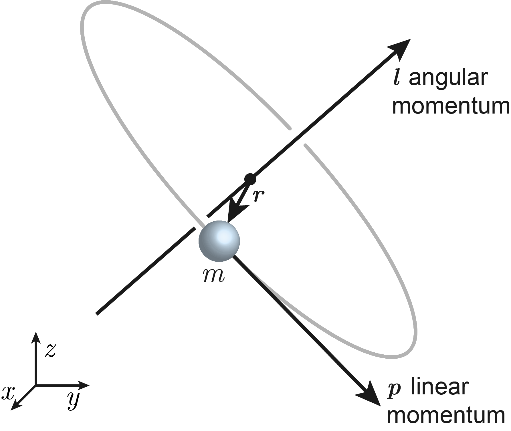
Figure 7.1 The definition of angular momentum \(\boldsymbol{l}\). It points along the rotation axis, following the right-hand rule.
The angular momentum vector can be written in terms of its components along three space-fixed perpendicular axes
where \(l_x\), \(l_y\), and \(l_z\) are the components of \(\boldsymbol{l}\) along the x, y, and z axis. The magnitude-squared of this vector is
There are two ways of writing the kinetic energy of a rotating body, either using the moment of inertia \(I\) and the angular frequency \(\omega\), or \(I\) and the angular momentum:
where the connection is through \(l = I\omega\).
7.2. Quantum angular momentum
The quantum angular momentum operator is obtained by replacing the linear momentum vector \(\boldsymbol{p}\) with its operator analog \(\hat{\boldsymbol{p}}\)
Replacing \(l^2\) with \(\hat{l}^2\) in the kinetic-energy expression above gives the Hamiltonian for a rotating body:
In the chapter on rotating molecules, we have solved the time-independent Schrödinger equation for this already. Therefore, the eigenfunctions of \(\hat{l}^2\) are the spherical harmonics \(Y_l^{m_l}(\theta,\phi)\), with eigenvalues \(\hbar^2 l(l+1)\):
with the quantum numbers \(l = 0,1,2,\dots\) and \(m_l=0,\pm1,\dots,\pm l\). This means that the magnitude of the angular momentum is quantized - only the discrete values \(\hbar\sqrt{l(l+1)}\) are possible measurement outcomes.
The spherical harmonics are also eigenfunctions of of the operator \(\hat{l}_z\) (the \(z\) component of \(\hat{\boldsymbol{l}}\)):
This means that, if one measures the angular momentum along an axis (call it \(z\)), then the only possible outcomes are multiples of \(\hbar\), \(\hbar m_l\). Since there are only discrete allowed projections along \(z\), the angular-momentum vector cannot point anywhere in space - it is confined to a cone for each \(m_l\) state. This is called space quantization.
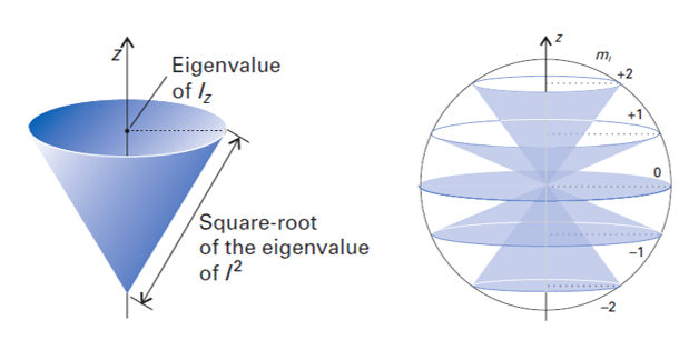
Figure 7.2 The vector model for quantum angular momentum. Left: The delocalization cone for a specific \((l,m_l)\) state. Right: Cones for all \((l,m_l)\) states with \(l=2\).
Figure 7.2 (left) depicts the vector model for an angular momentum state with quantum numbers \(l\) and \(m_l\). In this model, angular momentum is pictured as a vector of defined length \(\hbar\sqrt{l(l+1)}\) and defined projection \(m_l\hbar\) along the direction \(z\). To indicate the fact that the x and y components are indeterminate, a cone is drawn. The orientation of the angular-momentum vector is “delocalized” over this cone, i.e. the tip of the vector could be anywhere on the cone rim. This delocalization of orientation is analogous to the delocalization of position in the particle-in-a-box and the other model systems we looked at earlier. Figure 7.2 (right) shows the vector model for all states with \(l=2\) (d functions). In this case, the magnitude is \(\hbar\sqrt{6}\), and the projections are \(-2\hbar\), \(-\hbar\), 0, \(+\hbar\), and \(+2\hbar\).
Note
It is incorrect to read into the vector model that the vector is precessing on the cone! The cone represents the possible orientations the vector can be found in when measured. The vector is orientationally delocalized over the cone in the same sense as an electron is delocalized in space.
Commutation relations. The three components of the angular momentum do not commute:
With the uncertainty principle, this implies that there exists no quantum state where all three are uniquely and precisely defined (except for \(l=0\)). In contrast, the angular-momentum operator \(\hat{l}^2\) and \(\hat{l}_z\) do commute:
The angular-momentum operators commute with the Hamiltonian of a hydrogenic atom:
This indicates that, in addition to the energy, also the magnitude of the angular momentum, as well as its projection onto a direction, are conserved quantities (constants of motion). There is one quantum number per operator: \(n\), \(l\), \(m_l\). The wavefunctions of the stationary states of the hydrogen atom are simultaneous eigenfunctions of all three operators.
7.3. Spin angular momentum
In addition to orbital angular momentum due to its motion around the nucleus, an electron has an additional intrinsic angular momentum indicated by \(\boldsymbol{s}\). This is present even if the electron has no orbital angular momentum (e.g. in a 1s orbital). This intrinsic angular momentum is called spin angular momentum, or simply spin, since it is possible to picture it as being due to the electron spinning around its own axis.
The spin angular momentum of the electron is fixed and has a magnitude of \(\hbar \sqrt{3/4}\), corresponding to a half-integer quantum number, \(s=1/2\). It is fixed, meaning that it is not possible to stop or accelerate the spinning. The half-integer value of the quantum number \(s\) is in contrast to the orbital angular momentum quantum numbers \(l\), which are integers. The analog of the orbital projection quantum number \(m_l\) is the spin projection quantum number \(m_s\), with the two possible values \(+1/2\) and \(-1/2\). The state with \(m_s=+1/2\) is called spin-up and indicated by \(\alpha\), and the state with \(m_s=-1/2\) is called spin-down and indicated by \(\beta\). The vector model representation of these two states is shown in Figure 7.3.
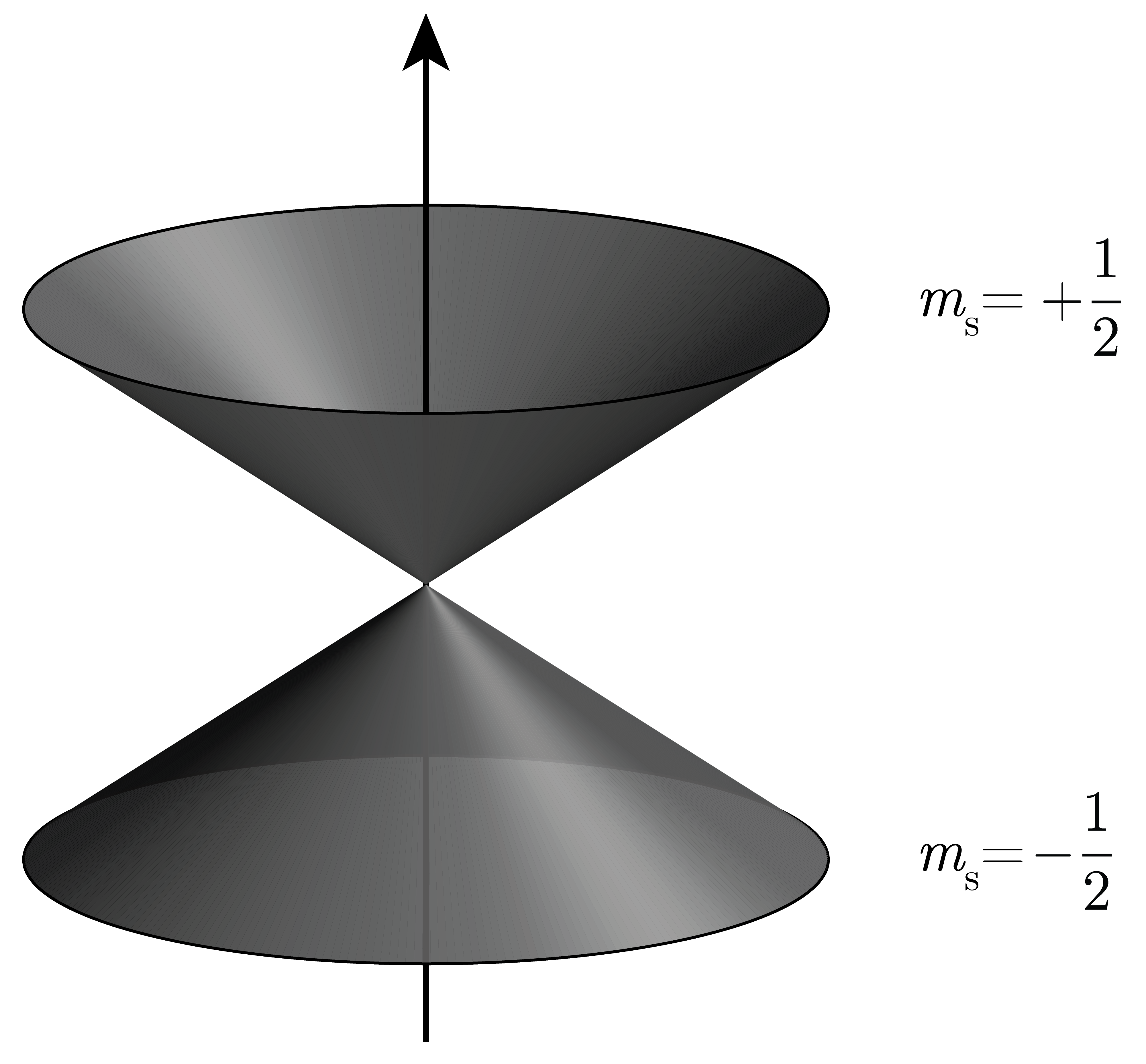
Figure 7.3 Vector model for the two stationary states of an electron spin: spin-up (\(\alpha\), \(m_s=+1/2\)) and spin-down (\(\beta\), \(m_s=-1/2\)). The fixed-length spin angular momentum vector is delocalized over the upper cone for the spin-up state, and over the lower cone for the spin-down state.
Aside from this difference in the quantum numbers, one further difference between orbital and spin angular momentum is that the spin eigenfunctions are not functions of continuous spatial variables (like \(\theta\) and \(\phi\)), but of the discrete coordinate \(m_s\) (which has the only possible values \(+1/2\) and \(-1/2\)). Some properties of spin and orbital angular momentum are summarized in the following table.
property |
orbital angular momentum |
spin angular momentum |
|---|---|---|
quantum numbers |
\(l=0,1,2,...\) and \(m_l = 0,\pm1,...,\pm l\) |
\(s=1/2\) and \(m_s = \pm1/2\) |
eigenfunctions |
\(Y_l^{m_l}(\theta,\phi)\) |
\(\alpha(m_s)\) and \(\beta(m_s)\) |
length |
\(\hbar\sqrt{l(l+1)}\) |
\(\hbar\sqrt{s(s+1)} = \hbar\sqrt{3/4}\) |
projection |
\(\hbar m_l\) |
\(\hbar m_s = \pm\hbar/2\) |
operators |
\(\hat{l}^2\), \(\hat{l}_x\), \(\hat{l}_y\), \(\hat{l}_z\) |
\(\hat{s}^2\), \(\hat{s}_x\), \(\hat{s}_y\), \(\hat{s}_z\) |
orthonormality |
\(\left\langle Y_{l'}^{m_l'}\middle|Y_l^{m_l}\right\rangle = \delta_{l',l}\delta_{m_l',m_l}\) |
\(\left\langle\alpha|\beta\right\rangle = \left\langle\beta|\alpha\right\rangle = 0\) \(\left\langle\alpha|\alpha\right\rangle = \left\langle\beta|\beta\right\rangle = 1\) |
The spin operators commute with the orbital operators and the Hamiltonian, so that there are a total of five commuting operators: \(\hat{H}\), \(\hat{l}^2\), \(\hat{l}_z\), \(\hat{s}^2\), and \(\hat{s}_z\).
Due to the spin of the electron, five quantum numbers are needed to fully specify an eigenstate of a hydrogenic atom: \(n\), \(l\), \(m_l\), \(s\), and \(m_s\). Since \(s\) is fixed, it is usually not explicitly listed, and only the remaining four quantum numbers are given. The total wavefunction \(\psi_{n,l,m_l,m_s}\) is the product of the spatial wavefunction and the spin function:
The spatial part \(\psi_{n,l,m_l}\) is called a spatial orbital, and the full wavefunction is called a spinorbital. In chemistry, spin orbital symbols are natural extensions of the symbols for spatial orbitals. For example, \(1\mathrm{s}\alpha\) indicates \(\psi_{1,0,0,+1/2}\), and \(3\mathrm{p}_z\beta\) indicates \(\psi_{3,1,0,-1/2}\).
Electrons are not the only particles that possess spin. Neutrons and protons (1H nuclei) are spin-1/2 particles. Since nuclei are composed of protons and neutrons, many nuclei (but not all) have non-zero spin angular momentum as well. The following table lists a few common nuclear isotopes and their nuclear spin quantum number, which is traditionally indicated by the letter \(I\).
Spin \(I\) |
Nuclear isotopes |
|---|---|
0 |
12C, 16O, 32S |
1/2 |
1H, 13C, 15N, 19F, 31P |
1 |
2H, 14N |
3/2 |
33S, 63Cu, 65Cu |
5/2 |
17O, 27Al, 55Mn |
7.4. Magnetic dipole moments
Both orbital and spin angular momenta of the electron give rise to a magnetic field. Therefore, electrons possess a magnetic dipole moment.
Orbital magnetic dipole moment. An electron with non-zero orbital angular momentum can be pictured as rotating around a nucleus. This represents a circular electric current, which produces a magnetic field. Therefore, an atom with an electron in an \(l\neq0\) state possesses an orbital magnetic dipole moment \(\boldsymbol{\mu}_l\) that is proportional to its orbital angular momentum. It is given by
where \(e\) is the (positive) elementary charge and \(m_\mathrm{e}\) is the mass of the electron. The dimension of \(\boldsymbol{\mu}_l\) is energy per field, and its SI unit is J T-1 (joule per tesla). Due to the negative charge of the electron, the electron magnetic dipole moment vector is antiparallel to the angular momentum vector, as indicated by the negative sign.
Spin magnetic dipole moment. An electron, with its non-zero spin angular momentum, can be pictured as a spinning negative charge. This is also equivalent to a circular electric current, and leads to a spin magnetic dipole moment:
The prortionality factor \(\gamma_\mathrm{e}\) is the gyromagnetic ratio of the electron and represents the ratio of magnetic moment to angular momentum. The \(g_\mathrm{e}\) factor is called the g factor of a free (unbound) electron. Its value depends on the local environment. For an unbound electron, it is about 2.00232.
Protons and other nuclei with non-zero spin also have a spin magnetic dipole moment.
where \(m_\mathrm{p}\) is the mass of the proton. The nuclear gyromagnetic ratio \(\gamma_\mathrm{n}\) and the nuclear g factor \(g_\mathrm{n}\) depend on the particular isotope. For example, \(g_\mathrm{n}\) is +5.58569 for a proton, +1.4048236 for a carbon-13 nucleus, and -0.56637768 for a nitrogen-15 nucleus.
7.5. Zeeman effect
When placed in an external magnetic field \(\boldsymbol{B}\), the energy of a magnetic dipole moment \(\boldsymbol{\mu}\) depends on its orientation relative to the field. Mathematically, its energy is the negative scalar product of the two vectors
where \(\theta\) is the angle between the two vectors. The energy is lowest if the magnetic moment is parallel to the field, and highest if it is antiparallel. This is illustrated in Figure 7.4.
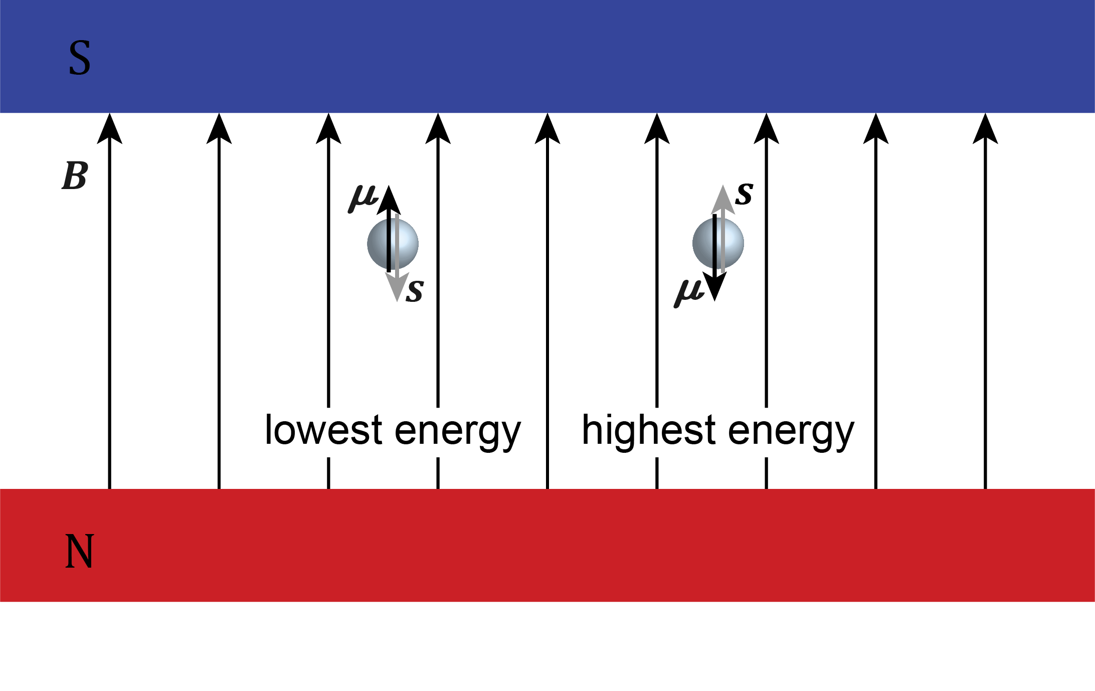
Figure 7.4 The energy of an electron in a magnetic field depends on the relative orientation between its magnetic moment \(\boldsymbol{\mu}\) and the magnetic field \(\boldsymbol{B}\).
The above equation also shows that the energy depends linearly on the strength of the external magnetic field. This magnetic-field dependence of the energy is called the Zeeman effect.
Note
Magnetic field strengths span a large range: The earth magnetic field is between 25 and 65 μT, depending on location. In NMR (nuclear magnetic resonance) spectroscopy, a 400 MHz spectrometer uses 9.4 T. In clinical MRI (magnetic resonance imaging), 1.5-3 T are used. A neodymium magnet can generate fields up to 1.4 T.
If we define the \(z\) axis along the applied magnetic field, the Hamiltonian describing the Zeeman interaction between the orbital magnetic moment of the electron and the magnetic field is
The associated eigenvalues are
The factor \(\mu_\mathrm{B} = e\hbar/2m_\mathrm{e}\) is called the Bohr magneton and is an atomic-scale unit for the magnetic moment (similar to the Bohr radius for atomic-scale lengths). Its value is listed in the Appendix.
The Hamiltonian and the eigenvalues for the electron spin are analogous:
The Zeeman effect is also operative for magnetic nuclei. The eigenvalues for a nuclear spin with spin angular momentum quantum number \(I\) (and \(m_I = -I,-I+1,...,+I\)) are
where \(\mu_\mathrm{N}\) is the nuclear Bohr magneton, a constant (see the Appendix for its value).
7.6. Spin-orbit coupling
An electron moving around nucleus sees a moving nuclear charge. From the point of view of the electron, this is equivalent to an electric current! Since an electric current generates a magnetic field, the electron feels a magnetic field. This field is
where \(\boldsymbol{E}\) is the electric field and \(\boldsymbol{v}\) is the velocity of the electron.
This field is purely internal to the atom, a result of the electron moving around a charged nucleus. It does not involve externally applied fields (as in the Zeeman effect).
Since the electron is magnetic as a result of its spin, it interacts with this magnetic field, i.e. its energy depends on the relative orientation between the magnetic field and the magnetic moment of the electron. This is the spin-orbit coupling (SOC). The associated Hamiltonian is
where \(\xi\) is a function of \(r\). This results in different energies depending on the relative orientation between spin and the orbital-angular-momentum-induced magnetic field. This is illustrated in Figure 7.5.
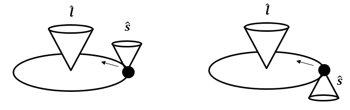
Figure 7.5 Spin-orbit coupling for an electron with orbital angular momentum \(\boldsymbol{l}\) and spin angular momentum \(\boldsymbol{s}\).
An important consequence of the spin-orbit coupling is now that the operators \(\boldsymbol{l}\) and \(\boldsymbol{s}\) don’t commute with the Hamiltonian anymore - they are not conserved quantities. However, the total angular momentum, denoted by \(\boldsymbol{j}\), is conserved. The total angular momentum is the vector sum of the orbital and the spin angular momentum:
The total angular momentum has the same properties as any other angular momentum: The eigenvalues of \(\hat{j}^2\) are \(\hbar^2 j(j+1)\) with \(j=0,1,2,\dots\), and the eigenvalues of \(\hat{j}_z\) are \(m_j = -j,-j+1,\dots,j\) for each \(j\).
The total number of states with given specific values of \(l\) and \(s\) can be determined as follows: for \(l\), we have \(2l+1\) states, and for \(s\), we have \(2s+1\) states. With \(s=1/2\), thus, the total is \(2(2l+1)\).
Note
The total number of states for a 2p electron (\(l=1\) and \(s=1/2\)) is obtained as follows. The number of orbital angular momentum states is \(2l+1 = 3\) (i.e. there are three different values of \(m_l\)), and the number of spin angular momentum states is \(2s+1=2\) (i.e. there are two different values of \(m_s\)). In total, that gives 3 times 2 = 6 states.
In order to determine the possible values of \(j\), we need to examine the possible \(m_l\) and \(m_s\), determine the associated \(m_j\), and then infer which \(j\) is associated with the \(m_j\) values.
If \(l=0\), then \(m_l=0\) and \(m_s=\pm1/2\), and we have two states total. The possible values for \(m_j\) are \(m_j=m_l+m_s=\pm1/2\). Such a range of \(m_j\) can only be due to \(j = 1/2\), (2 states). All states are accounted for.
If \(l=1\), then \(m_l=-1,0,1\) and \(m_s=\pm1/2\), and we have a total of 6 combinations of \(m_l\) and \(m_s\). We can classify them according to the value of \(m_j\), as shown in the following table:
\(m_j\) |
\((m_l,m_s)\) |
no. of states |
\(j=3/2\) |
\(j=1/2\) |
|---|---|---|---|---|
\(+3/2\) |
\((1,1/2)\) |
1 |
1 |
|
\(+1/2\) |
\((1,-1/2)\), \((0,1/2)\) |
2 |
1 |
1 |
\(-1/2\) |
\((0,-1/2)\), \((-1,1/2)\) |
2 |
1 |
1 |
\(-3/2\) |
\((-1,-1/2)\) |
1 |
1 |
There is one state with \(m_j=+3/2\). Since this is the largest \(m_j\), we can conclude that there is a group of states with \(j=3/2\), with 4 states (\(m_j=+3/2\), \(+1/2\), \(-1/2\), \(-3/2\)). If we remove these states, we are left with one \(m_j=1/2\) state and one \(m_j = -1/2\) state. These can only be due to \(j=1/2\) (2 states, \(m_j=\pm1/2\)). Therefore, the coupling of the 6 states with \(l=1\) and \(s=1/2\) yields one set of 4 states with \(j=3/2\) and one set of 2 states with \(j=1/2\).
The above are special cases of the general rule for the addition of angular momenta. For one electron, the possible values of \(j\) are
(if \(l=0\), these two are identical). For \(l=1\) and \(s=1/2\), this directly gives \(j=1/2\) and \(j=3/2\).
For several electrons, the orbital and spin angular momenta of the individual are combined first to give \(L = \sum_k l_k\) (orbital) and \(S = \sum_k s_k\) (spin), and then \(L\) and \(S\) are combined to give the total angular momentum \(J\), with the possible values
For each \(J\), there are \(2J+1\) states (\(m_J = -J,\dots,J\)). For example, \(L=2\) and \(S=1\) will give \(J=1\), 2, and 3 terms with 3, 5, and 7 states. This type of coupling is called Russell-Saunders coupling. For a one-electron atom, \(J=j\), \(L=l\), and \(S=s=1/2\).
A group of \(2J+1\) states with the same \(J\) is called a term and is identified by a term symbol. It represents information about the spin, orbital, and total angular momentum. The general notation for a term symbol is
The pre-superscript indicates the spin multiplicity and is called spin singlet for \(2S+1=1\), spin doublet for \(2S+1=2\), spin triplet for \(2S+1=3\), etc. A one-electron atom has \(S=s=1/2\) and \(2S+1=2\), so it is a spin doublet. \(X\) is a letter representing \(L\): S (\(L=0\)), P (1), D (2), F (3), etc. \(J\) is the total angular momentum quantum number.
Note
The term symbols for the one-electron configurations in a hydrogen atom are
1s: \(^2\mathrm{S}_{1/2}\)
2s: \(^2\mathrm{S}_{1/2}\)
2p: \(^2\mathrm{P}_{3/2}\), \(^2\mathrm{P}_{1/2}\)
If the electron is in a 2p state, this indicates that there are two different terms (groups of states) with different total angular momenta.
Note
A \(^4\mathrm{D}_{5/2}\) term indicates a group of states with spin angular momentum \(S=3/2\) (pre-superscript \(2S+1=4\)), orbital angular momentum \(L=2\) (letter D), and total angular momentum \(J=5/2\) (subscript). The term consists of \(2J+1=6\) states.
7.7. Fine structure of H atom
Figure 7.6 shows the consequences of spin-orbit coupling (SOC) for the energy levels hydrogen atom. On the left, SOC is neglected, and all states of the 2p electron configuration are degenerate. The SOC coupling causes a splitting between the two terms of 2p configuration, the lower-energy term being \(^2\mathrm{P}_{1/2}\) (2 degenerate states), and the higher-energy term being \(^2\mathrm{P}_{3/2}\) (4 degenerate states). Instead of a single emission line, the 2p\(\rightarrow\)2s transition consists in reality of two lines that are very close together. If a magnetic field is applied in addition, the states within the two terms split due to the Zeeman effect, and there are many emission lines with (very slightly) different wavelengths.
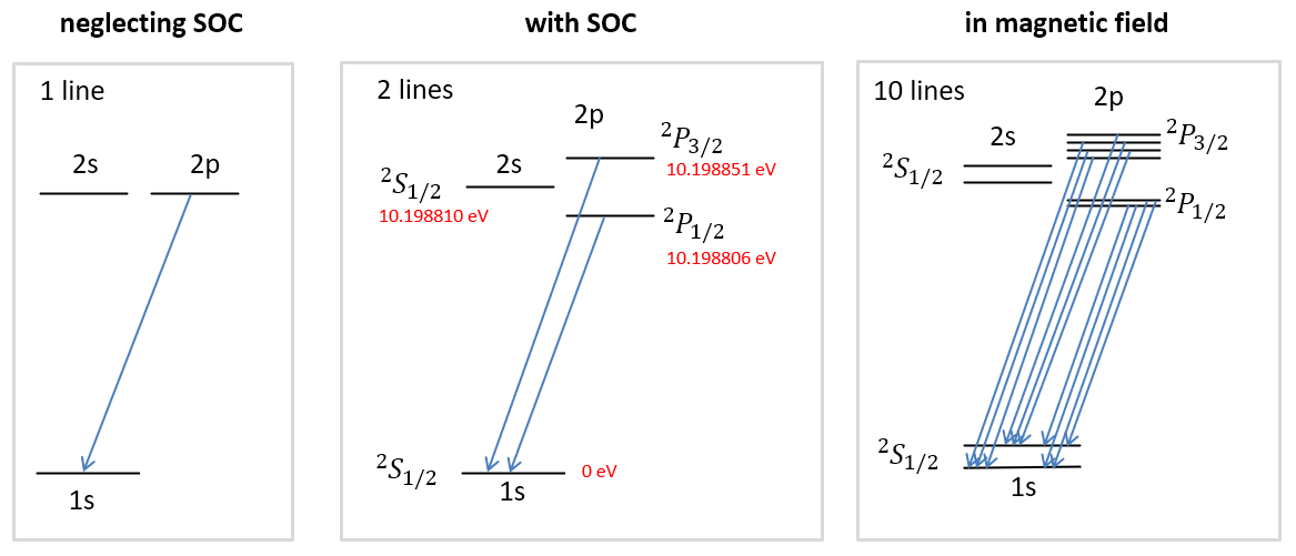
Figure 7.6 The fine structure of the hydrogen atom. Spin-orbit coupling leads to a splitting of the 2p states into \(^2\mathrm{P}_{1/2}\) (2 degenerate states) and \(^2\mathrm{P}_{3/2}\) (4 degenerate states). Application of a magnetic field removes all degeneracies.
The selection rules for transitions are \(\Delta L = \pm1\), \(\Delta S = 0\), \(\Delta J = 0,\pm1\), and \(\Delta m_J = 0,\pm1\).
The selection rule \(\Delta S = 0\) is of particular importance. It indicates that only transitions between spin singlet states, or between spin triplet states, are possible. Transitions between states of different spin multiplicity (such as from a triplet state to a singlet state) are called spin-forbidden and are very unlikely.
7.8. Magnetic resonance
The Zeeman effect is the basis of magnetic resonance spectroscopy (MR): nuclear magnetic resonance (NMR) spectroscopy and magnetic resonance imaging (MRI) for nuclei (predominantly 1H), and electron paramagnetic resonance (EPR) spectroscopy for (unpaired) electrons.
There are two crucial differences between MR and other spectroscopies such as UV/vis and infrared spectroscopy. First, the sample is placed in an external static magnetic field in order to split the Zeeman states energetically. Without a field, the Zeeman states would be degenerate. The splitting between the energy levels increases linearly with the field strength. Second, magnetic-resonance transitions are induced by the the oscillating magnetic-field component of the incident radiation, rather than the electric-field component (see introductory chapter). The magnetic-field component exerts a torque (a rotating force) on the magnetic dipole moment and rotates it in space.
Selection rules. In magnetic resonance, the selection rule is that transitions are observed (“allowed”) only if the projection quantum number changes by one unit, i.e.
for NMR and EPR, respectively.
The energy of such an allowed transition is
for EPR and NMR, where either the g-factors \(g_\mathrm{e}\) and \(g_\mathrm{n}\) (both unitless) are used or the gyromagnetic ratios \(\gamma_\mathrm{e}\) and \(\gamma_\mathrm{n}\) (with SI unit rad s-1 T-1).
Figure 7.7 shows the energy level diagram of a proton (1H nucleus) as a function of the strength of an applied magnetic field. To represent energies \(E\), in MR it is common to use the frequency equivalent, \(E/h\).
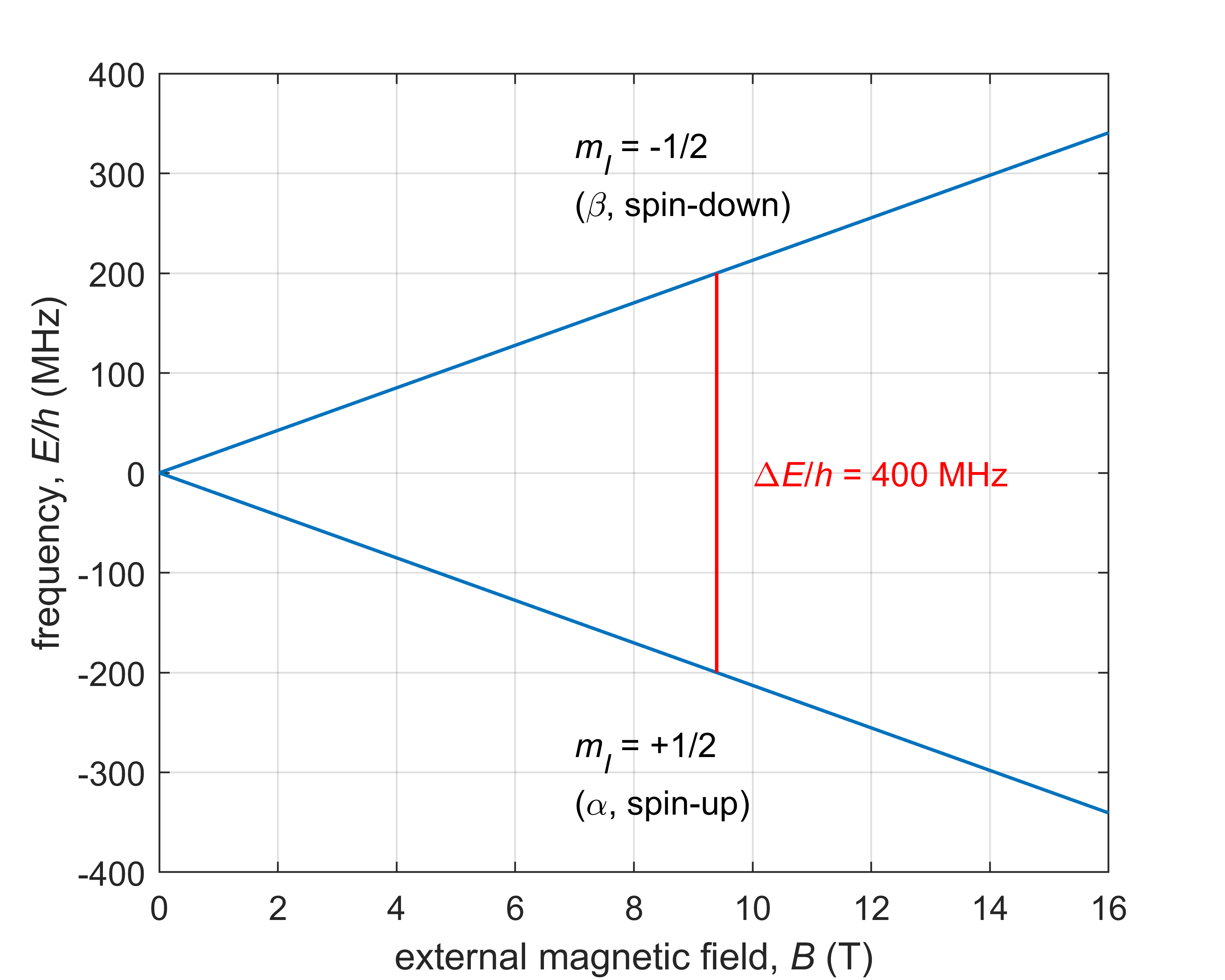
Figure 7.7 The Zeeman energy level diagram for a proton in an external magnetic field, with the allowed transition indicated.
Note
A typical NMR spectrometer operates with a field of 9.39 T, at which protons absorb at a frequency of about 400 MHz (which corresponds to a photon energy of 1.6 µeV). Typical EPR spectrometers operate around 0.3 T, with frequencies of 9 to 10 GHz (37-41 µeV).
Chemical shifts. The exact value of the g-factor (or gyromagnetic ratio) depends on the local atomic and molecular enviroment of the electron or nucleus. A naked electron, outside any atom or molecule, has a g-factor of 2.00232. In a molecule, this value is shifted to larger or smaller values, as a result of local magnetic fields that are induced by the applied magnetic field. These local fields either reinforce or counteract the externally applied field, such that the magnetic particle experiences an amplified or attenuated overall field. For unpaired electrons, spin-orbit coupling is the main mechanism for this shift.
Note
In NMR, the chemical shifts are relatively small. The shifts are measured relative to protons and 13C in the reference compound TMS (tetramethylsilane, Si(CH3)4) and are on the range of 0-10 ppm (parts per million) for protons, and 0-220 ppm for 13C.
In EPR, the chemical shifts are generally much larger. The g-factor for an unpaired electron in a Cu(II) complex can be as large as 2.4, which is a 20% (200,000 ppm) shift from 2.0023. In organic radicals, g values are typically between 2.0023 and 2.01, corresponding to shifts of up to 0.4% (about 5000 ppm).