3. Translational motion

In this chapter, we apply quantum theory to a series of model situations: a single particle confined to one-, two-, or three-dimensional microscopic “boxes”, i.e. regions where it can move freely, but beyond which it cannot move. The purpose of studying these simple systems is to examine many of the concepts and predictions of quantum concepts closely, without the hassle of mathematical complications. These insights then apply to much more complex systems such as atoms and molecules as well.

3.1. Particle in a 1D box

The simplest quantum system is a single particle moving freely along a single dimension within a finite region. This system is often referred to as a particle in a box. Despite its simplicity, this turns out to be an approximate model for predicting the color of linear organic molecules with extended conjugated pi systems (linear polyenes).

In the particle-in-a-box model, a single particle of mass \(m\) is free to move along one dimension (\(x\)), but with its motion restricted to a finite region (called the “box”) \(0\le x\le a\), where \(a\) is the length of the box (see Figure 3.1). Macroscopic analogs are a car on rails, a bead on a string, or a ball in a tube or pipe.

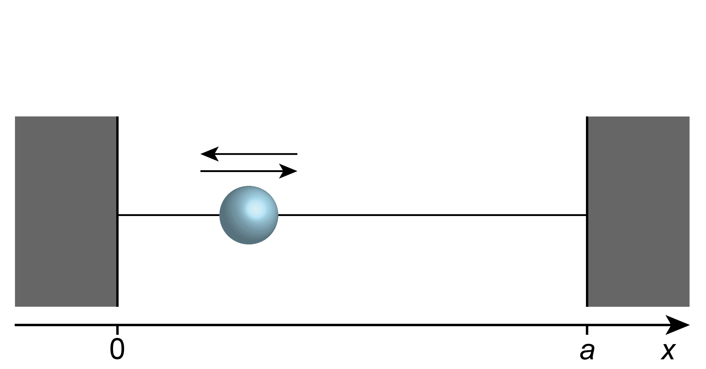
Figure 3.1 The particle-in-a-box model.

Mathematically, the limitation of the range of motion is represented by choosing an apropriate potential-energy function, \(V(x)\). Within the box, where the particle can move freely, the potential energy is constant. The value of this constant does not affect the solution, and for mathematical convenience we can set it to zero, \(V(x) = 0\). In order to represent the impossibility for the particle to be outside box, the potential energy outside the box is set infinitely large, \(V(x)=\infty\). Together:

(3.1)\[\begin{split}V(x) = \begin{cases} 0 & \quad \text{for } 0\le x\le a\\ \infty & \quad \text{everywhere else} \end{cases}\end{split}\]

This potential-energy function is illustrated in Figure 3.2. It is the reason why this system is often referred to as “infinitely deep potential well”.

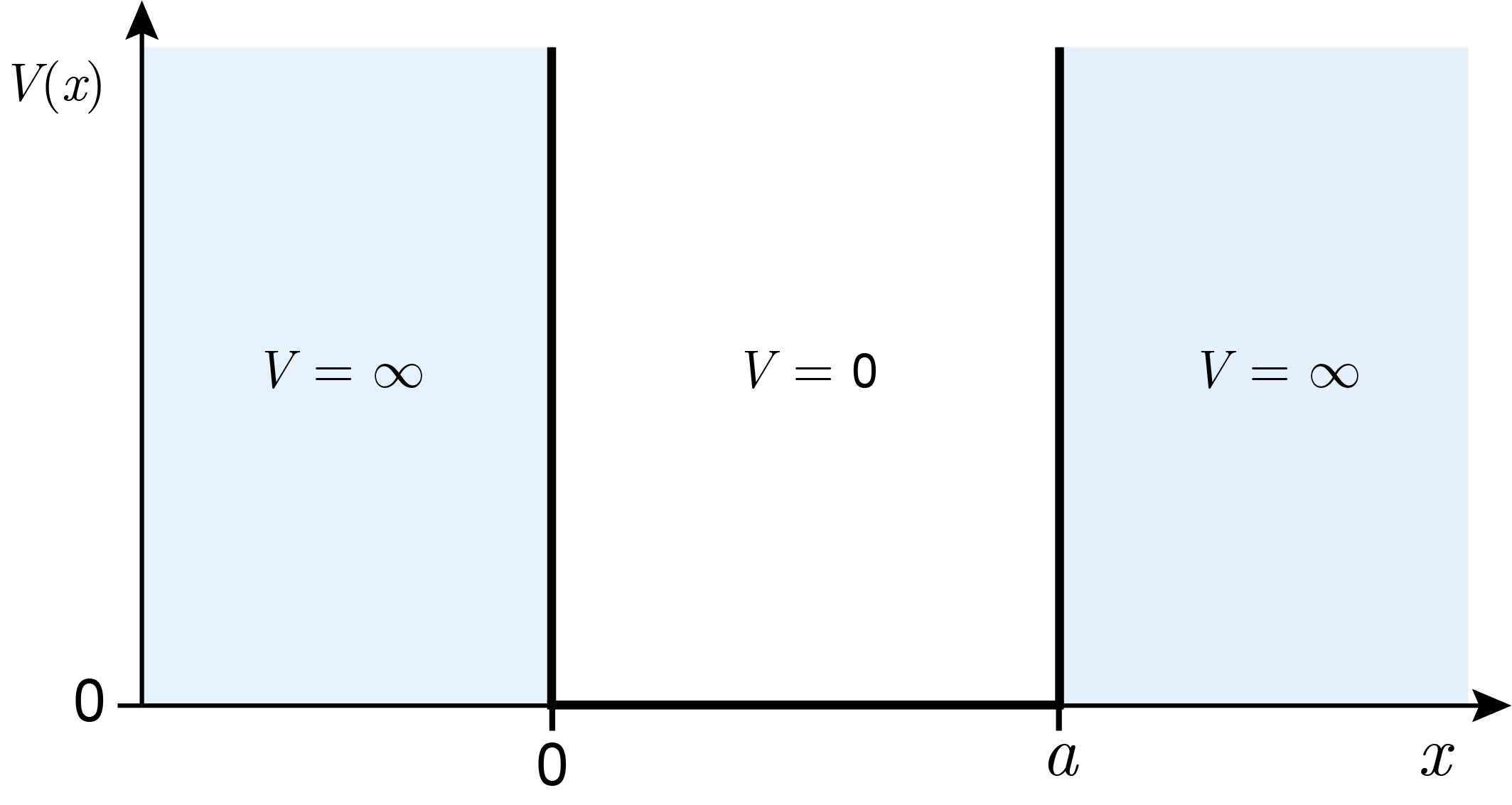
Figure 3.2 The potential function for a quantum particle in a 1-dimensional box.

A macroscopic particle without kinetic energy in a macroscopic box would just be at rest at some position within the box, and with some kinetic energy it would move alternately to the left and to the right, bouncing off the two potential “walls” at \(x=0\) and \(x=a\) and reversing direction.

To get insight into the behavior of a microscopic particle in a microscopic box, we need to determine and examine the wavefunctions describing the stationary states. For this, we need to set up the Hamiltonian and then solve the time-independent Schrödinger equation.

Outside the box, this is not necessary, as per definition there should be zero probability of finding the particle. Therefore, \(\psi(x) = 0\) everywhere outside the box. Inside the box, the potential energy is zero (\(\hat{V}=0\)), and the Hamiltonian for this region is

(3.2)\[\hat{H} = \hat{T} + \hat{V} = \hat{T} = -\frac{\hbar^2}{2m}\frac{\mathrm{d}^2}{\mathrm{d}x^2}\]

where \(m\) is the mass of the particle. The associated time-independent Schrödinger equation reads

(3.3)\[-\frac{\hbar^2}{2m}\frac{\mathrm{d}^2}{\mathrm{d}x^2}\psi(x) = E\cdot\psi(x)\]

Solving it will give us the wavefunctions \(\psi\) and the associated energies \(E\). To get there, we first multiply by \(-2m/\hbar^2\) and introduce the abbreviation

(3.4)\[k^2 = 2mE/\hbar^2\]

This yields

(3.5)\[\frac{\mathrm{d}^2}{\mathrm{d}x^2}\psi(x) = -k^2\psi(x)\]

This is a second-order differential equation with the general mathematical solutions \(\psi(x) = c_1\sin(kx)+c_2\cos(kx)\), with the two arbitrary coefficients \(c_1\) and \(c_2\). Although all \(\psi\) of this form satisfy the equation mathematically, not all of them are physically valid. Since a physical \(\psi\) must be continuous, and \(\psi\) must be zero outside the box, it must also be zero at the box boundaries \(x=0\) and \(x=a\). At \(x=0\), this requirement leads to

(3.6)\[\psi(0) = c_2\cos(k\cdot 0) = c_2 \qquad\rightarrow\qquad c_2 = 0\]

At \(x=a\), this means

(3.7)\[\psi(a) = c_1\sin(ka) = 0\]

\(c_1\) cannot be zero, since then the entire wavefunction would vanish, and there would be no particle anywhere. Therefore, \(\sin(ka)\) must be zero, which is the case only if \(ka\) is a multiple of \(\pi\): \(ka = n\pi\) for \(n=0,\pm1,\pm2,\dots\) Now, \(n\) cannot be zero, because then again the entire wavefunction would vanish. Negative values of \(n\) lead to an overall sign change of the function (since \(\sin(-n\pi x/a) = -\sin(n\pi x/a)\)), and wavefunctions that differ only in their overall sign are fully equivalent. Therefore, we can disregard negative values of \(n\). The boundary condition at \(x=a\) therefore results in

(3.8)\[k = \frac{n\pi}{a}\qquad\text{ for }n=1,2,3,\dots\]

This means that only for these specific \(k\) values there are physically valid solutions among the mathematical solutions. With this, the physically valid wavefunctions have the general form \(\psi(x) = c_1\sin(n\pi x/a)\). If we require the wavefunction to be normalized, then \(c_1\) assumes a specific value. We can determine it from the normalization requirement

(3.9)\[\langle\psi|\psi\rangle = \int_{-\infty}^{\infty}|\psi|^2\mathrm{d}x \stackrel{!}{=} 1\]

Carrying out the integral yields \(|c_1|^2 = 2/a\). If we choose \(c_1\) to be real and positive, this gives \(c_1 = \sqrt{2/a}\). The general form for the wavefunction solutions is

(3.10)\[\psi_n(x) = \sqrt{\frac{2}{a}}\sin\left(n\pi \frac{x}{a}\right) \qquad n = 1,2,3,\dots\]

\(n\) is called the quantum number. We have added a subscript \(n\) to \(\psi\) to indicate its dependence on \(n\).

These wavefunctions are the eigenfunctions of \(\hat{H}\). The associated energy eigenvalues are obtained by rearranging \(k^2 = 2mE/\hbar^2\) to \(E = k^2\hbar^2/2m\) and combining this with \(k = n\pi/a\). This gives

(3.11)\[E_n = \frac{\pi^2 \hbar^2}{2m a^2}\cdot n^2 = \frac{h^2}{8ma^2}\cdot n^2 \qquad n = 1,2,3\dots\]

Again, we added a subscript \(n\) to indicate that the energy depends on the quantum number \(n\). This indicates that only certain energies are possible in the sense that only these values are obtainable when the energy of a particle in a box is measured. The energies are illustrated in Figure 3.3. Note that there is only one state for each energy level, indicating that all states are non-degenerate.

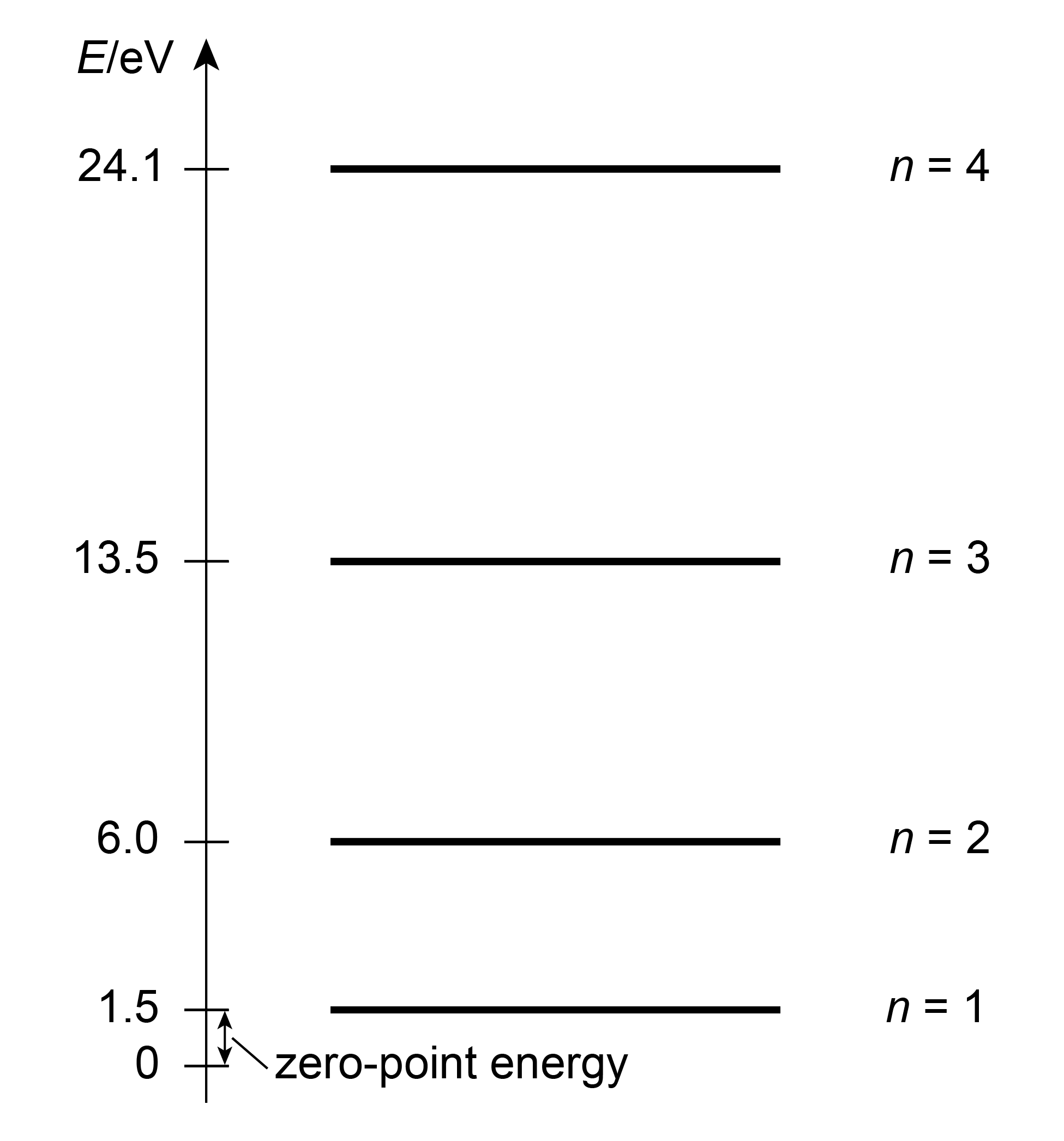
Figure 3.3 The energies of a particle in a 1D box.

A few important properties of \(E_n\) should be noted. First, the energy of the ground state (\(n = 1\)) is non-zero. This energy consists of kinetic energy only (the potential energy is zero), and we can calculate the associated speed of the particle by equating \(E_n\) to the kinetic energy \(mv^2/2\):

(3.12)\[\frac{h^2}{8ma^2}n^2 = \frac{1}{2}mv^2 \qquad \rightarrow \qquad |v| = \frac{h}{2ma}n\]

This signifies that even in the lowest possible energy eigenstate, the particle is still moving - quite remarkable. The non-vanishing energy in the ground state, in this case kinetic energy only, is called the zero-point energy (ZPE).

Second, the energies \(E_n\) grow quadratically with \(n\). Third, for a given \(n\), the kinetic energy and therefore the speed of the particle decreases with increasing box size \(a\) and increasing mass \(m\).

The wavefunctions are shown in Figure 3.4. They are all real-valued and oscillatory and resemble standing waves. The number of half-waves is equal to \(n\): The wavefunction for the ground state (\(n=1\)) consists of one half-wave, the one for \(n=2\) of two half-waves, and so on. The number of zero crossings (nodes) in the wavefunction increases with increasing \(n\): none for \(n=1\), one for \(n=2\), etc. This is a result of the faster oscillations with higher \(n\). The increasing curvature (second derivative) indicates increasing kinetic energy.

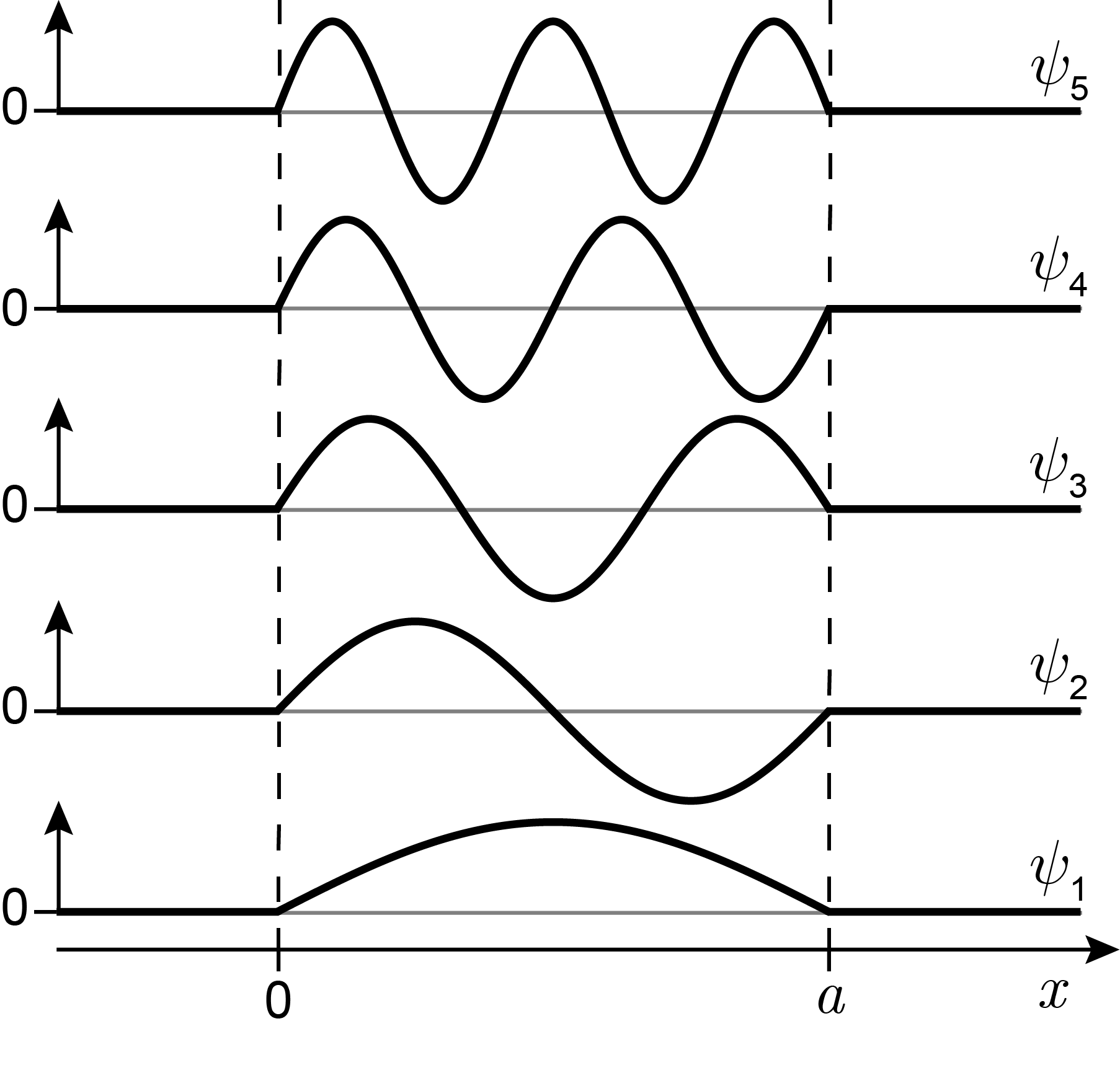
Figure 3.4 The wavefunctions for a particle in a 1D box in the lowest few energy eigenstates.

Also, note that the wavefunctions have alternating symmetry with respect to the center of the box at \(x=a/2\). Wavefunctions with odd \(n\) (1, 3, …) are symmetric with respect to the center, and wavefunctions with even \(n\) (2, 4, …) are antisymmetric.

Note that these wavefunctions are single-valued, square integrable, and continuous (no discontinuities). However, they are not smooth, as they have a discontinuous first derivatives (kinks) at \(x=0\) and \(x=a\). In principle, this means the function is non-physical. In this particular case, however, the potential energy jumps to infinity, and the resulting kink in \(\psi_n\) is acceptable.

The probability densities \(|\psi_n|^2\) for the various states are shown in Figure 3.5. They show of a series of \(n\) evenly spaced peaks, with zeroes in between and at the box edges. This indicates that the probability of finding a particle is highly position-dependent. For example, \(|\psi_1|^2\) indicates that in the ground state it is more likely to find the particle near the center of the box than near one of the edges.

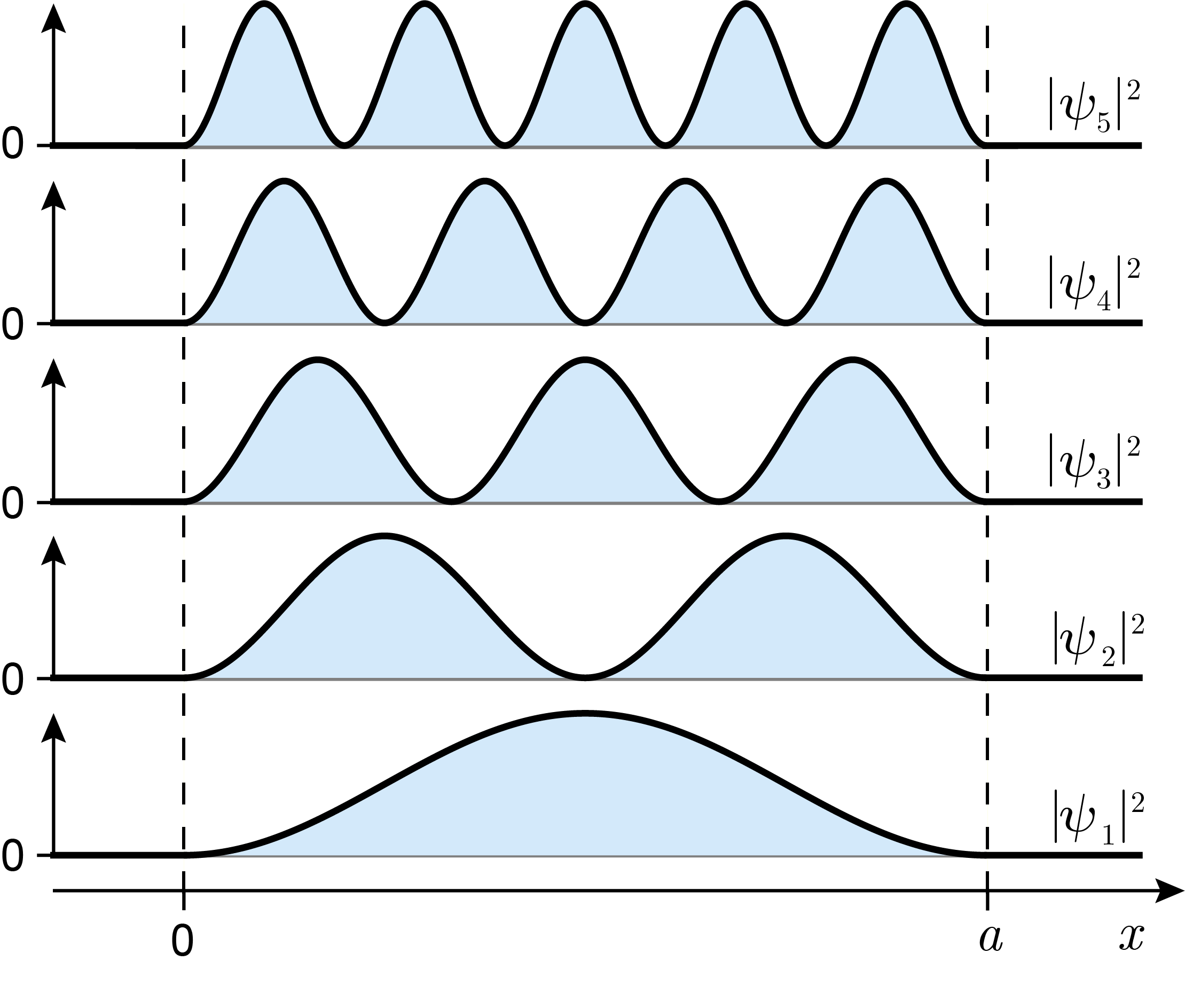
Figure 3.5 The probability densities for various states of a particle in a 1D box.

Let’s examine some of the properties of the wavefunctions. They should be pairwise orthogonal (for \(m\neq n\)), since they are eigenfunctions of a Hermitian operator. Explicitly, we can check this with the integral

(3.13)\[\langle\psi_m|\psi_n\rangle = \int_{-\infty}^\infty \psi_m^*\psi_n \mathrm{d}x = \frac{2}{a} \int_0^a \sin\left(m\pi\frac{x}{a}\right) \sin\left(n\pi\frac{x}{a}\right) \mathrm{d}x\]

which evaluates to zero for \(m\neq n\). Since each \(\psi_n\) is also normalized, the wavefunctions form an orthonormal set: \(\langle\psi_m|\psi_n\rangle = \delta_{m,n}\). The set is complete in the sense that any other function \(\psi\) can be expressed as a linear combination (superposition) of \(\psi_n\):

(3.14)\[\psi(x) = \sum_{n=1}^\infty c_n\psi_n(x)\]

Functions of this form are called superposition wavefunctions. They are not eigenfunctions of the energy (Hamiltonian) and do not satisfy the time-independent Schrödinger equation. However, they do satisfy the time-dependent Schrödinger equation and are therefore describe physically possible states. The states corresponding to these superposition wavefunctions are non-stationary and change as a function of time. Figure 3.6 shows an example of a superposition wavefunction. Energy measurements on such a state have several possible outcomes, with associated probabilities given by \(|c_n|^2\) (assuming \(\psi\) is normalized).

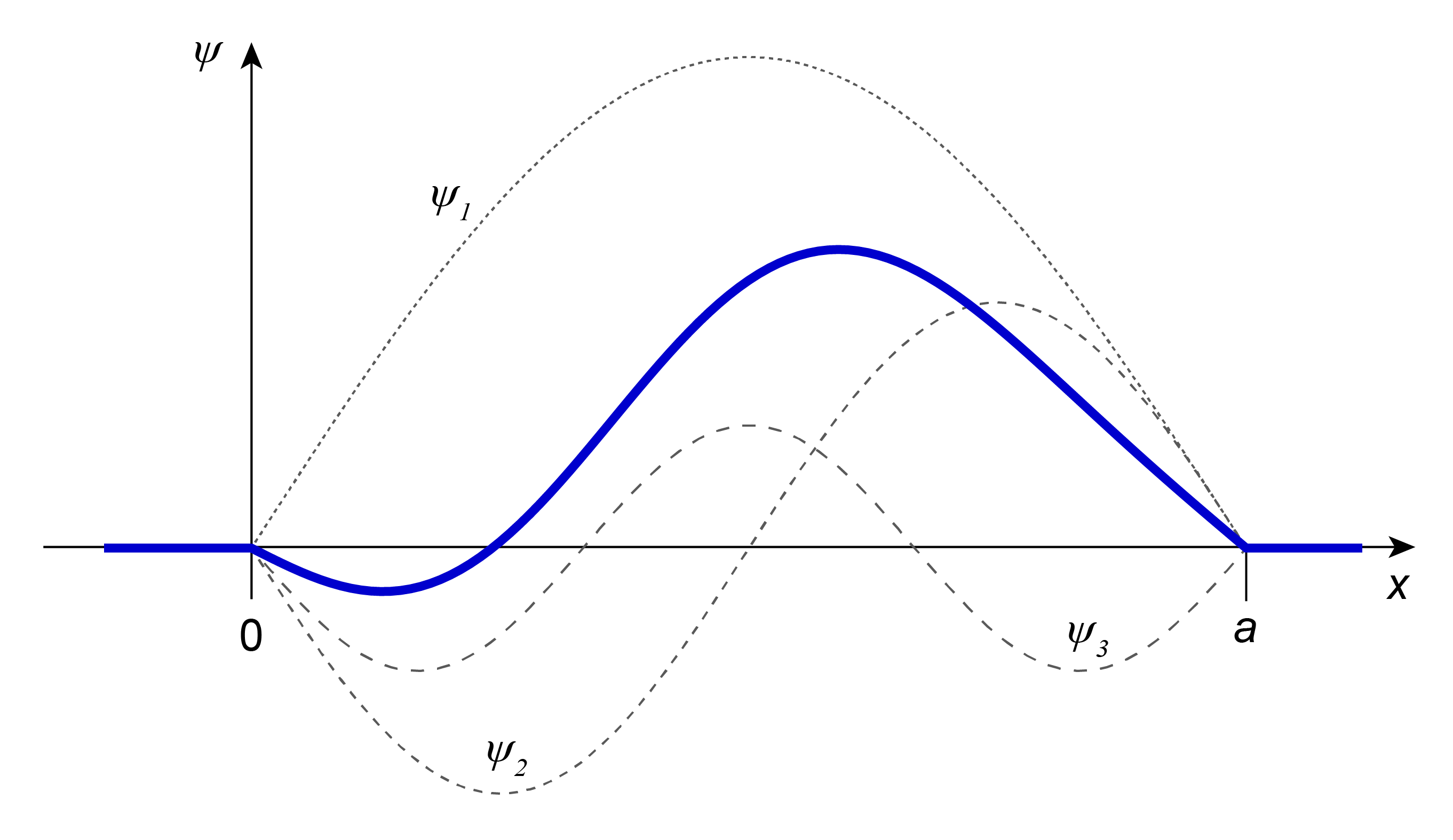
Figure 3.6 An example of a superposition wavefunction, \(\psi \propto 2\psi_1 - \psi_2 - \psi_3/2\), describing a non-stationary state with non-unique energy.

Note

Energy of a superposition wavefunction. Take a particle in a 1D box in a state described by the superposition wavefunction

(3.15)\[\psi(x) = \frac{2}{\sqrt{13}}\psi_1(x) - \frac{3}{\sqrt{13}}\psi_5(x)\]

where \(\psi_1\) and \(\psi_5\) are the normalized energy eigenfunctions with \(n=1\) and \(n=5\).

There are three things we can predict about energy measurements:

• The possible outcomes of an energy measurement are \(E_1 = h^2/8ma^2\) and \(E_5 = 25h^2/8ma^2\).

• The probabilities for these outcomes are \(4/13\) and \(9/13\), respectively.

• The energy expectation value for this wavefunction is

  (3.16)\[\langle E\rangle = \langle\psi|\hat{H}|\psi\rangle = \int_0^a\psi^*\hat{H}\psi\,\mathrm{d}x = \cdots = \frac{4}{13}E_1 + \frac{9}{13}E_5 = \frac{h^2}{8ma^2}\frac{229}{13} \approx 17.6\frac{h^2}{8ma^2}\]

3.2. Describing molecules

The simple model of a single particle in a one-dimensional box demonstrates the fundamentals of quantum theory, but does by itself not have any predictive power for any real-world situation. However, if we generalize it to multiple particles, it can be applied to linear conjugated molecules (linear polyenes). Such molecules have a quasi-linear network of carbon atoms connected by alternating single and double bonds. Each double bond contributes two \(\pi\) electrons, which are essentially freely mobile over the entire length of the molecule. It turns out that if we model the \(\pi\) electrons as confined in a simple 1D box, we can predict the absorption wavelengths, and thereby the color, of these molecules. Figure 3.7 shows two examples of naturally occurring linear polyenes.

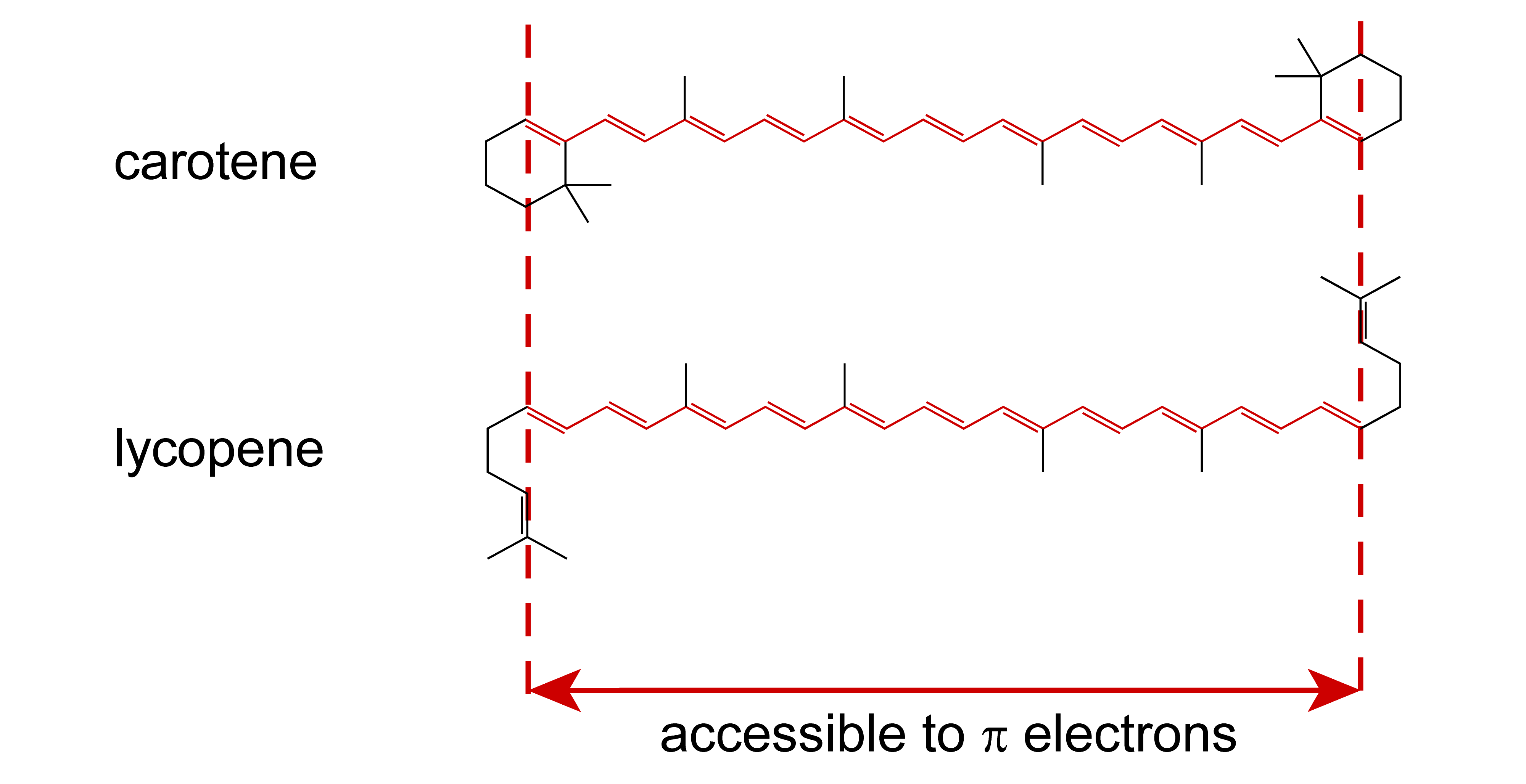
Figure 3.7 Carotene and lycopene, the main color pigments from carrots and tomatoes. The conjugated \(\pi\) system extends over 21 bonds (22 carbon atoms) and contains 22 \(\pi\) electrons.

To apply the particle-in-a-box model to many electrons, we need two additional concepts: the electron spin and the Pauli exclusion principle.

In addition to their translational degrees of freedom (\(x\), \(y\), \(z\) in three dimensions), electrons have an internal degree of freedom: spin angular momentum, or simply called spin. You can picture an electron as a small spherical particle spinning around an axis that goes through its center-of-mass - a motion that is analogous to the earth’s rotation around its north-south axis. The spinning frequency of the electron is universal and unchangeable, and the spin angular momentum is \(\hbar/2\). When the orientation of the spinning axis is measured, one of only two possible directions can be found: spin-up (\(\alpha\)) or spin-down (\(\beta\)). This internal degree of freedom is indicated by the letter \(m\), and its two possible values are \(m=+1/2\) and \(m=-1/2\). In contrast to the continuous translational degrees of freedom (\(x\) etc.), spin is a discrete degree of freedom.

The overall wavefunction of an electron is the product of a spatial part and a spin part. In one dimension:

(3.17)\[\begin{split}\psi(x,m) = \begin{cases} \psi(x)\cdot\alpha(m) \\ \psi(x)\cdot\beta(m) \end{cases}\end{split}\]

Now we can introduce some important terminology that links quantum theory to basic chemistry: the spatial part \(\psi(x)\) of this one-electron wavefunction is called a (spatial) orbital; the one-electron wavefunction \(\psi(x,m)\), including both spatial and spin parts, is called spin-orbital. A molecular orbital (MO) is a one-electron wavefunction in a molecule, and an atomic orbital (AO) is a one-electron wavefunction in an atom.

In order to model multiple electrons in the same quantum system, we need to adhere to the Pauli exclusion principle, which states that two electrons can never be in the same state (i.e. never be described by the same one-electron wavefunctions). This principle applies to all particles with spin 1/2 (electrons, protons, neutrons, and others), which are called fermions.

Note

According to the Pauli exclusion principle, it is possible to have a two-electron system with the two electrons in states \(\psi_1\alpha\) and \(\psi_1\beta\), but impossible to have both of them in state \(\psi_1\alpha\).

Next, let us model multiple electrons in the same box. If we neglect, for now, the electrostatic repulsion between the electrons and treat them as independent particles, we can then just fill the energy level diagram from bottom to top to get the overall ground state. This results in a series of occupied and unoccupied MOs. For example, in 1,3-butadiene there are 4 \(\pi\) electrons, and therefore we fill \(\psi_1\alpha\), \(\psi_1\beta\), \(\psi_2\alpha\), and \(\psi_2\beta\). The highest occupied MO (HOMO) is \(n=2\), and the lowest unoccupied MO (LUMO) is \(n=3\).

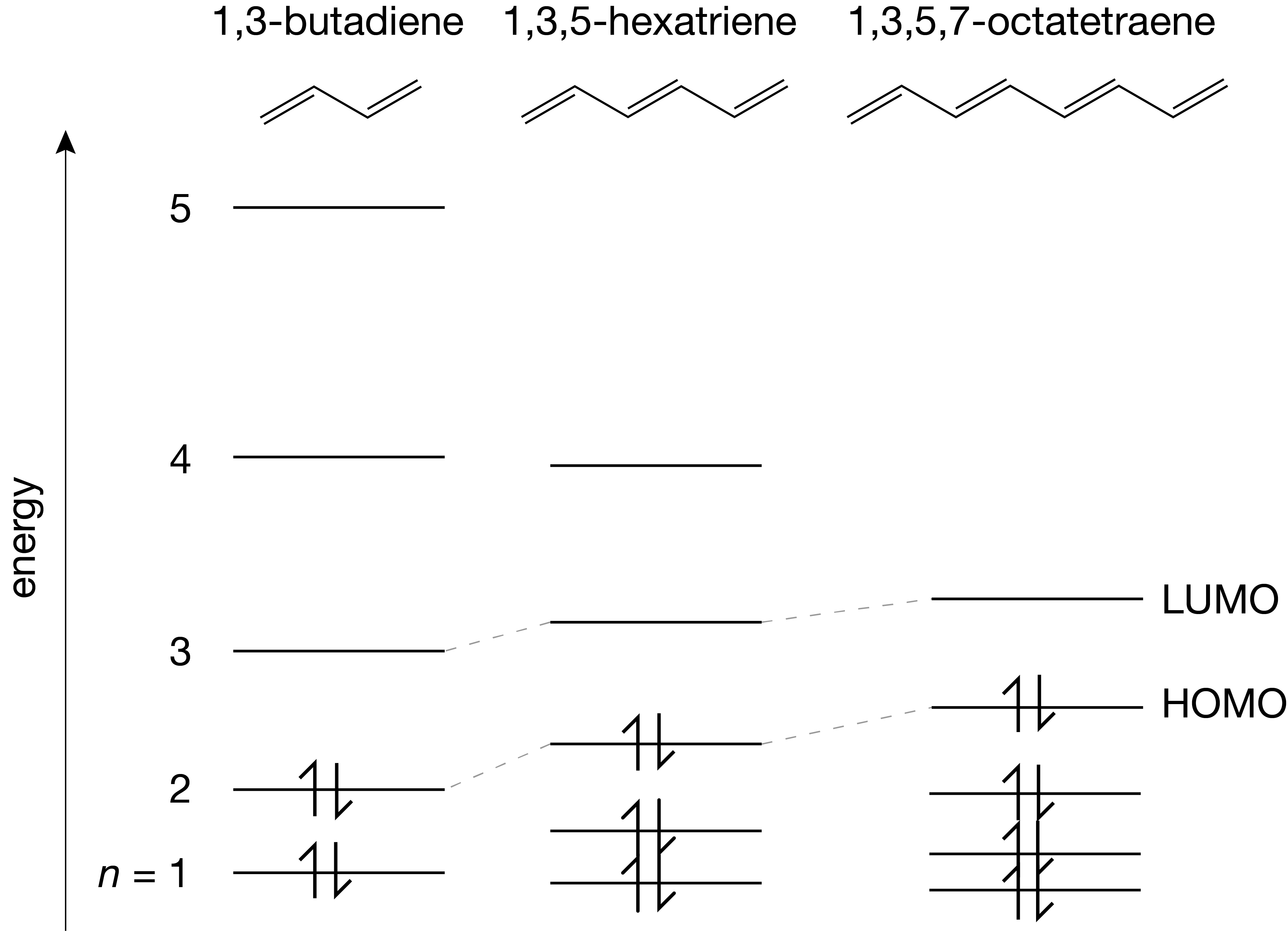
Figure 3.8 The particle-in-a-box model applied to simple linear polyenes.

Light can be absorbed by this molecule only at wavelengths where the photon energy matches the energy difference between an occupied MO and an unoccupied MO. This absorption is accompanied by the promotion of the electron from the occupied to the unoccupied MO, resulting in the transition of the molecule from the lower-energy state to an higher-energy state. Of particular interest is the longest-wavelength (lowest-energy) transition, since for many molecules it lies in, or close to, the visible range of the electromagnetic spectrum. This transition corresponds to the HOMO-LUMO transition. Assuming the HOMO has quantum number \(n\), the transition energy is

(3.18)\[\Delta E = E_{n+1}-E_n = \frac{h^2}{8ma^2}\left[(n+1)^2-n^2\right] = \frac{h^2}{8ma^2}\left(2n+1\right)\]

To calculate the absorption wavelength, we equate this energy difference to the photon energy:

(3.19)\[\Delta E = E_\mathrm{photon} = \frac{hc}{\lambda} \qquad \rightarrow \qquad \lambda = \frac{8mc}{h}\frac{a^2}{2n+1}\]

This equation predicts the absorption wavelengths surprisingly well.

Note

Let us apply the particles-in-the-box model to carotene (see Figure 3.7), in order to predict its absorption wavelength. We assume the box extends over the 21 carbon-carbon bonds, and we assume the molecule is fully extended. With an average bond length of \(r_{CC} = 140\,\mathrm{pm}\) and a bond angle of \(\alpha = 124^\circ\), the box length is \(a = 21 r_{CC}\sin(\alpha/2) = 2.60\,\mathrm{nm}\). Carotene has 11 pairs of \(\pi\) electrons, occupying the 11 lowest \(\pi\) MOs. The HOMO is \(n=11\), and the LUMO is \(n=12\). The \(n = 11\rightarrow 12\) transition has an energy difference of \(\Delta E = 1.28\,\mathrm{eV}\). The predicted absorption wavelength is \(\lambda = 966\,\mathrm{nm}\). Experimentally, the absorption maximum is at about \(480\,\mathrm{nm}\). The model predicts this within a factor of 2, which is remarkable given the simplicity of the model.

It is important to realize that the electrons-in-a-box model is very approximate and makes a series of serious approximations: (a) It is one-dimensional, but electrons move in three dimensions. (2) The potential inside the box is assumed flat, but in molecules, there is periodicity due to the underlying carbon-carbon bond network. (3) The potential outside the box is assumed infinite, but in reality we can knock out an electron from the molecule and ionize it using sufficiently high photon energies. (4) The model is limited to \(\pi\) electrons only, but there are many more electrons in the molecule. (5) It is assumed that electrons are independent. However, they repel each other, raising the overall potential energy. Also, their positions are correlated - if one electron is in the left side of the box, the others will tend to be on the right side due to repulsion.

Despite these limitations, the particle-in-a-box model is useful for qualitative reasoning. For example, Figure 3.9 shows that the number of half-waves and nodes in the 1D model correspond to the number of lobes and nodal planes in the three-dimensional MOs.

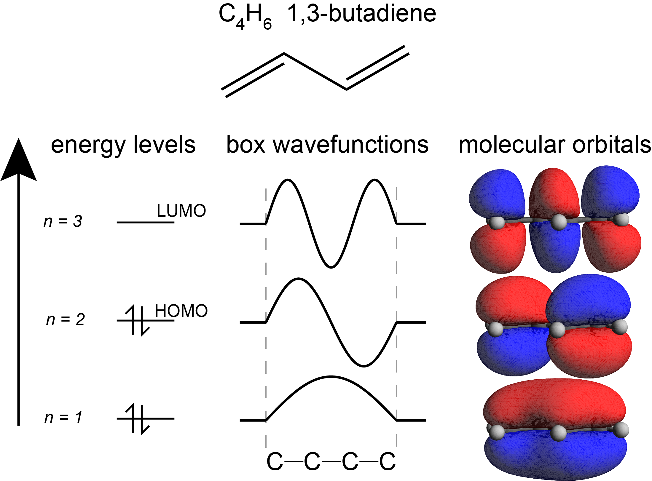
Figure 3.9 The frontier molecular orbitals of butadiene, compared to the particle-in-a-box model.

3.3. Multi-dimensional potential wells

So far, we examined situations where a particle (or particles) are constrained to move in a one-dimensional region (potential well). We can apply the same method to describe particles in two- and three-dimensional potential wells.

For a two-dimensional box with lengths \(a\) and \(b\), the potential-energy function is

(3.20)\[\begin{split}V(x,y) = \begin{cases} 0&\text{for } 0\le x\le a\text{ and } 0\le y \le b\\ \infty&\text{otherwise} \end{cases}\end{split}\]

It is illustrated in Figure 3.10.

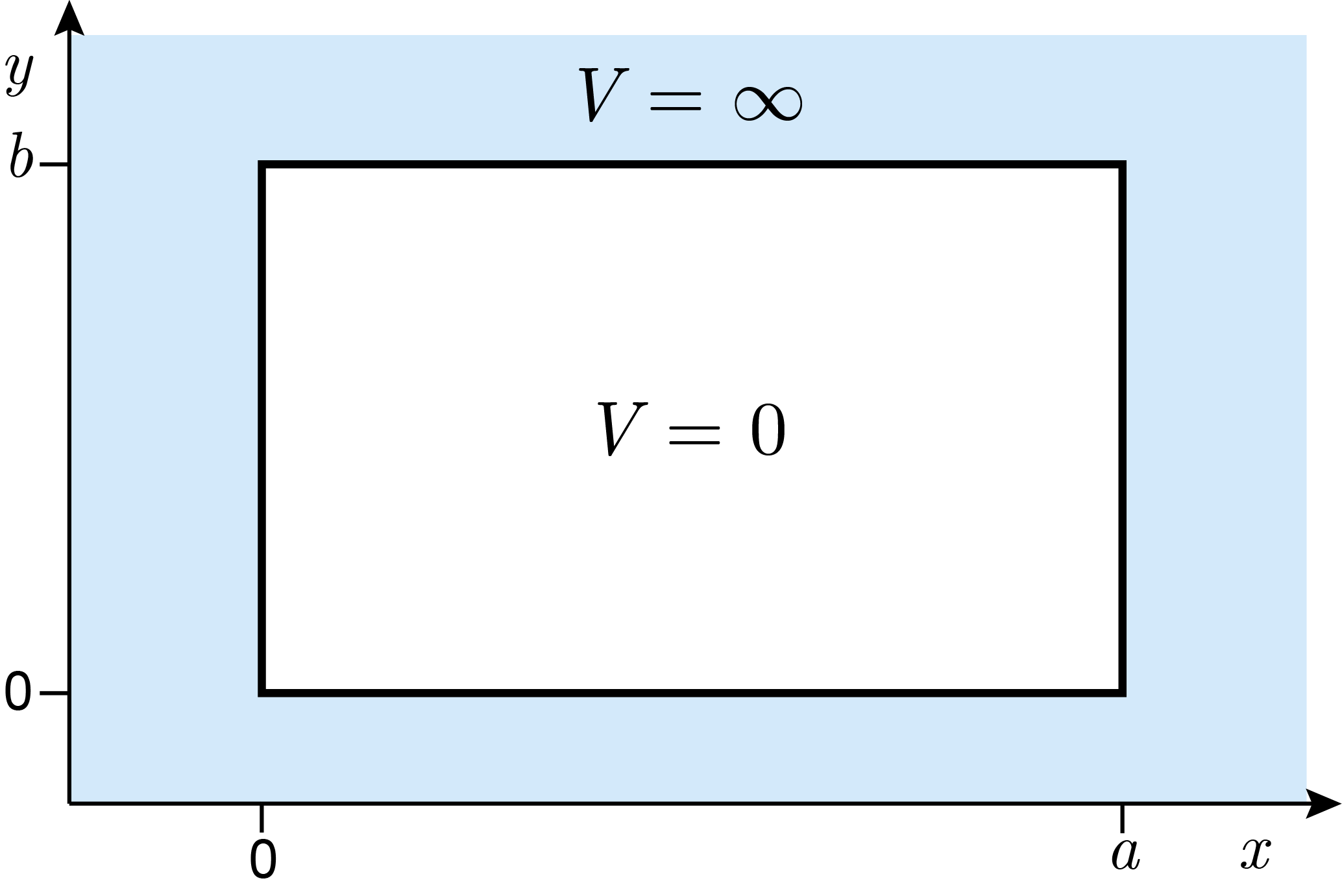
Figure 3.10 The potential energy of a two-dimensional box with edge lengths \(a\) and \(b\).

The time-independent Schrödinger equation for the region within the box is

(3.21)\[\hat{H}\psi(x,y) = -\frac{\hbar^2}{2m}\nabla^2\psi(x,y) = -\frac{\hbar^2}{2m} \left( \frac{\partial^2}{\partial x^2} + \frac{\partial^2}{\partial y^2} \right) \psi(x,y) = E\psi(x,y)\]

To solve this equation for \(\psi\), we can apply the method of separation of variables by using the following product ansatz (initial assumption)

(3.22)\[\psi(x,y) = X(x)\cdot Y(y)\]

where \(X\) and \(Y\) are functions that we need to determine. Inserting this into the Schrödinger equation, pulling unaffected quantities out of the derivatives, and dividing by \(\psi = X Y\) gives

(3.23)\[-\frac{\hbar^2}{2m} \left( \frac{1}{X} \frac{\partial^2 X}{\partial x^2} + \frac{1}{Y} \frac{\partial^2 Y}{\partial y^2} \right) = E\]

Each of the coordinates \(x\) and \(y\) can be varied independently. Varying \(x\) potentially changes the first term on the left-hand side, and varying \(y\) might change the second term. Now, the two terms have to add up to the same constant, no matter what values \(x\) and \(y\) assume. Therefore, each of the two terms must be by itself a constant. This means we have two separate equations:

(3.24)\[\begin{split}\begin{align} -\frac{\hbar^2}{2m} \frac{1}{X} \frac{\partial^2 X}{\partial x^2} &= E_x \\ -\frac{\hbar^2}{2m} \frac{1}{Y} \frac{\partial^2 Y}{\partial y^2} &= E_y \end{align}\end{split}\]

where we have decomposed the overall constant \(E\) into \(E_x + E_y\). Each of these equations is identical to the one used to solve the one-dimensional problem. Therefore, we can immediately write down the solutions for the energies \(E_x\) and \(E_y\) as well as for the wavefunctions \(X(x)\) and \(Y(y)\). The total energy is

(3.25)\[E_{n_x,n_y} = \frac{h^2}{8ma^2}n_x^2 + \frac{h^2}{8mb^2}n_y^2 = \frac{h^2}{8m} \left( \frac{n_x^2}{a^2} + \frac{n_y^2}{b^2} \right)\]

The energy depends on the two quantum numbers \(n_x\) and \(n_y\) (each with possible values 1, 2, 3, etc.), one for each degree of freedom. This is a general principle that is valid for systems with many particles in multiple dimensions: There is one quantum number per degree of freedom.

Figure 3.11 shows the energy level diagrams for two different 2D boxes differing in their aspect ratio (relative edge lengths).

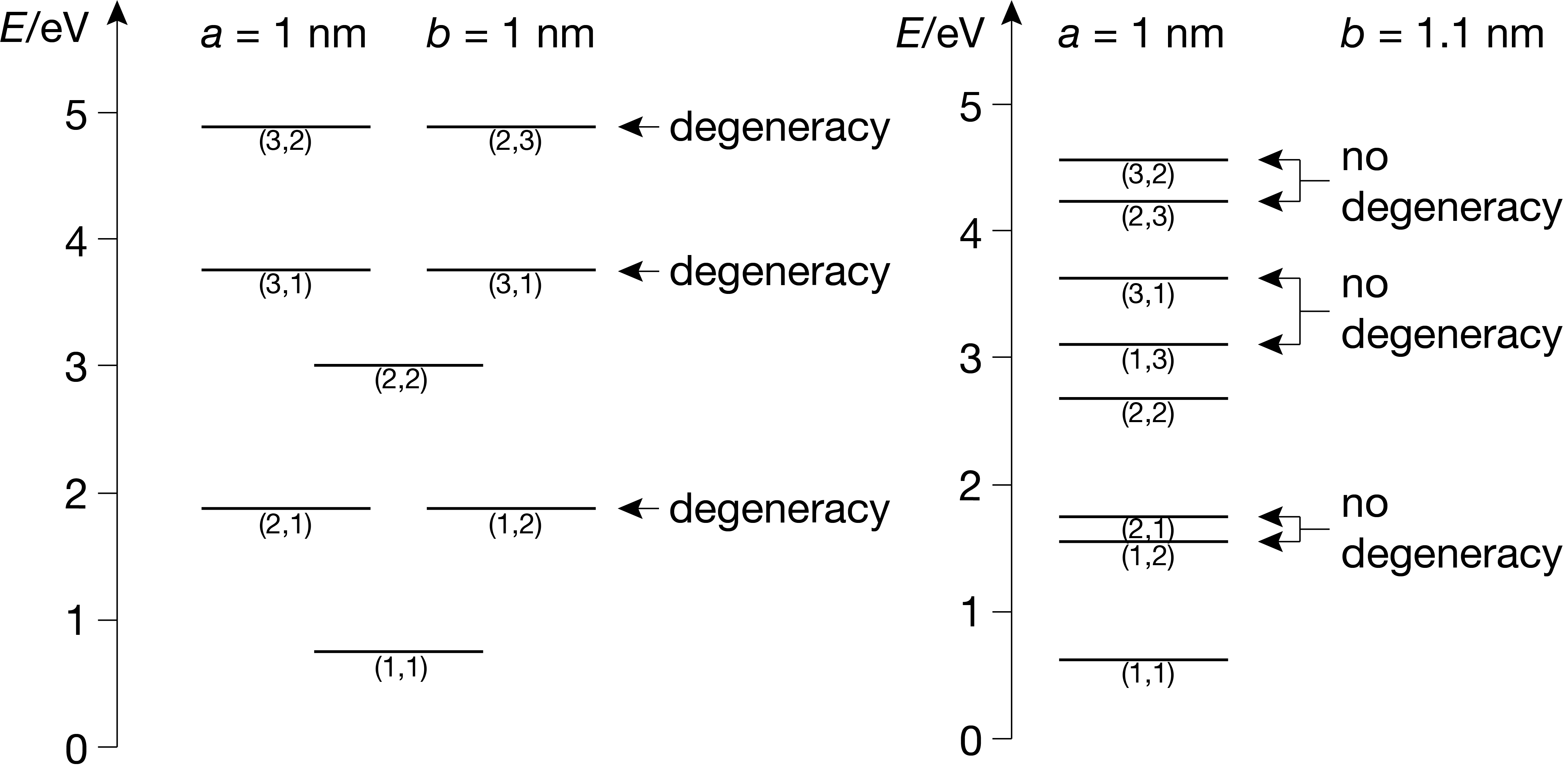
Figure 3.11 Energy level diagrams for a square 2D box (left) and a 2D box without symmetry (right).

The energy level diagram for the square box (\(a=b\)) shows multiple levels with doubly degenerate states. As soon as the high symmetry of the square box is broken by slightly changing one edge length, the degeneracies disappear. This is one instance of a more general principle: The higher the symmetry of the system, the more degeneracies appear.

The wavefunctions for the particle in the 2D box also depend on the two quantum numbers \(n_x\) and \(n_y\) and are the product of two 1D-box wavefunctions, one for each dimension:

(3.26)\[\psi_{n_x,n_y}(x,y) = \sqrt{\frac{4}{ab}}\cdot \sin\left(n_x\pi\frac{x}{a}\right) \sin\left(n_y\pi\frac{y}{b}\right)\]

Figure 3.12 shows the wavefunctions of the ground state \((n_x,n_y)=(1,1)\) and of the excited state with \((n_x,n_y) = (3,2)\).

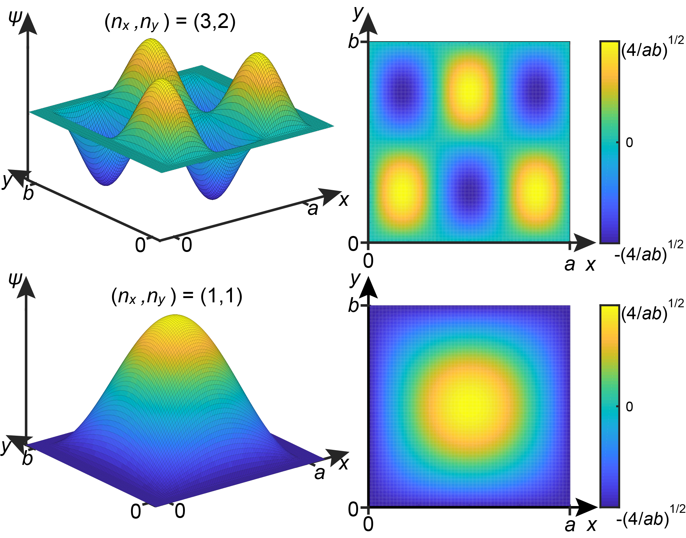
Figure 3.12 Examples of wavefunctions for the 2D box.

The method and results for the two-dimensional box generalize in a very straightforward way to a particle in a three-dimensional box. Assuming a box with edge lengths \(a\), \(b\), and \(c\) in the region \(0\le x\le a\), \(0\le y\le b\), and \(0\le z\le c\), the energies are sums of three contributions, one for each degree of freedom:

(3.27)\[E_{n_x,n_y,n_z} = \frac{h^2}{8m} \left( \frac{n_x^2}{a^2}+ \frac{n_y^2}{b^2}+ \frac{n_z^2}{c^2} \right)\]

Figure 3.13 shows the energy level diagram for a cubic box (\(a=b=c\)).

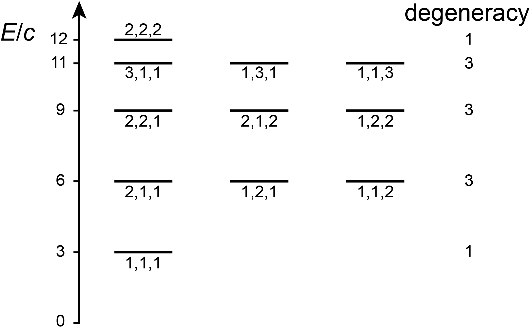
Figure 3.13 Energy level diagram for a particle in a cubic box. The constant \(c\) is \(h^2/(8ma^2)\). All state energies are labeled by the three quantum numbers \(n_x\), \(n_y\), and \(n_z\).

The associated wavefunctions are products of one-dimensional functions, again one for each degree of freedom:

(3.28)\[\psi_{n_x,n_y,n_z}(x,y,z) = \sqrt{\frac{8}{abc}}\cdot \sin\left(n_x\pi\frac{x}{a}\right) \sin\left(n_y\pi\frac{y}{b}\right) \sin\left(n_z\pi\frac{z}{c}\right)\]

Note

General principle. If the Hamiltonian is a sum of terms with separated variables, then its energy eigenvalues are sums of terms, and the associated wavefunctions are products of terms.

3.4. Finite-depth potential well

Next, we consider a quantum system with a particle and a potential well (a box) with finite depth \(V_0\). The potential-energy function is

(3.29)\[\begin{split}V(x) = \begin{cases} 0 &\text{ for } |x|\le a/2\\ V_0 &\text{ for } |x|>a/2 \end{cases}\end{split}\]

and is shown in Figure 3.14. (The \(x\) range is shifted relative to what we used previously. This is for mathematical convenience and is otherwise inconsequential.)

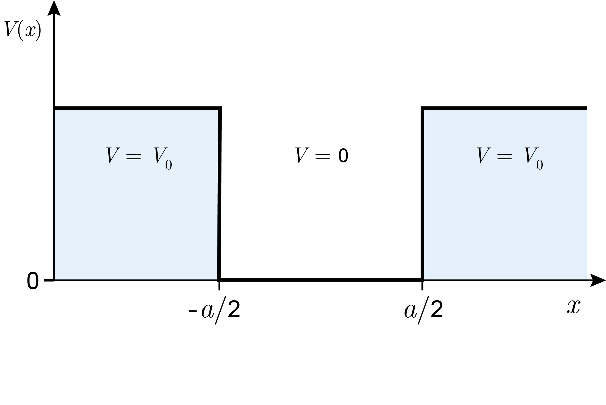
Figure 3.14 The potential-energy function for a finite-depth potential well.

There are two different types of situations, based on the total energy \(E\) of the particle relative to \(V_0\):

• \(E\ge V_0\). The energy \(E\) of the particle is larger than the well depth \(V_0\). In this case, the particle is not trapped and can move freely outside the well. The associated states are called unbound states.

• \(E<V_0\). The particle’s energy is smaller than the well depth. In this case, the particle is trapped inside the well. The associated states are referred to as bound states.

The number of bound states can be estimated using the expression for the energies from the infinitely deep potential well. The highest possible energy that still corresponds to a bound state is just below the potential well depth \(V_0\), so that

(3.30)\[\frac{h^2}{8ma^2}n_\mathrm{max}^2\approx V_0 \qquad \rightarrow \qquad n_\mathrm{max} \approx \frac{2a\sqrt{2mV_0}}{h}\]

Note

For an electron in a potential well of width 0.9 nm and depth 10.0 eV, we estimate about \(n_\mathrm{max}=4.6\approx5\) bound states. In fact, there are 5.

To quantitatively determine the energies and wavefunctions of the stationary bound states, we need to solve the time-independent Schrödinger equation. The details are given in the Appendix. First, all functions that mathematically solve for the Schrödinger equations for each of the three regions are found. Then, the physical boundary conditions (square integrability, continuity, and smoothness) are imposed, which selects the subset of functions that are physically acceptable wavefunctions. From the physical boundary conditions, equations for the energies are obtained. However, they cannot be solved analytically, and one has to resort to numerical methods.

The next figure shows an example of the resulting energies. They are indexed with a quantum number \(n\). However, keep in mind that there is no explicit equation that allows one to calculate an energy for a given \(n\).

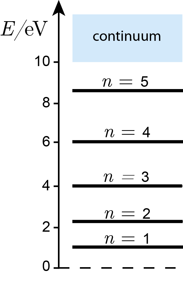
Figure 3.15 The energy for an electron in a potential well of 10 eV depth and 0.9 nm width.

The corresponding wavefunctions are shown in Figure 3.16. Inside the potential well, the wavefunctions are oscillatory of the form \(\cos(kx)\) (for odd \(n\)) or \(\sin(kx)\) (for even \(n\)). They have an increasing number of half-waves just as in the infinitely deep potential well: The ground state has one half-wave, the first excited state has two, etc. The wavefunctions with odd \(n\) (including the one for the ground state) are symmetric with respect to the center, whereas wavefunctions with even \(n\) are antisymmetric.

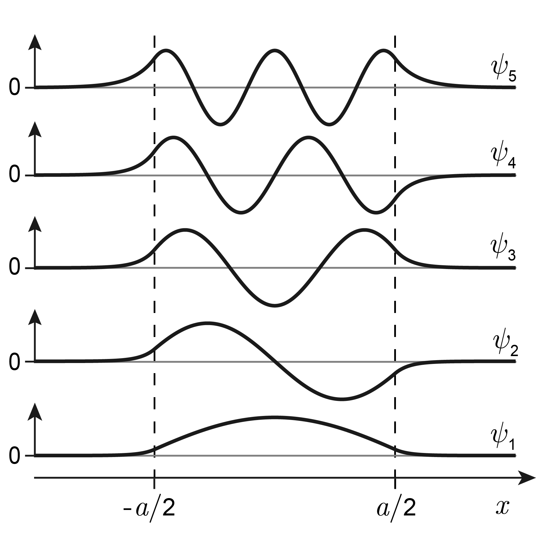
Figure 3.16 The wavefunctions for a particle in a finite-depth potential well.

Outside the box, the wavefunctions are non-zero and have the form of decaying exponentials. This behavior is in contrast to the infinitely deep well, where the wavefunctions reached exactly zero at the edges of the well. It also is in disagreement with classical (pre-quantum) physics, which predicts that this region should be inaccessible, since the energy of the particle \(E\) is smaller than the potential energy \(V_0\). Therefore, this region is commonly called “classically forbidden”. This is a surprising and counterintuitive quantum effect. Quantum theory predicts that particles can be found in regions where they shouldn’t be based on classical energy considerations!

The decaying exponentials are of the form \(\mathrm{exp}(\pm x/d)\), with the decay length, or penetration depth, \(d\). This describes how far into the classically forbidden region the particle can penetrate

(3.31)\[\text{penetration depth} = d = \frac{\hbar}{\sqrt{2m(V_0-E)}}\]

where \(E<V_0\). The closer \(E\) to \(V_0\), the smaller the denominator, and the longer the penetration depth. This can be seen in Figure 3.16: Wavefunctions with higher energy have more extended exponential tails than lower-energy wavefunctions.

Note

Ionization energy, photoelectric effect, photoelectron spectroscopy

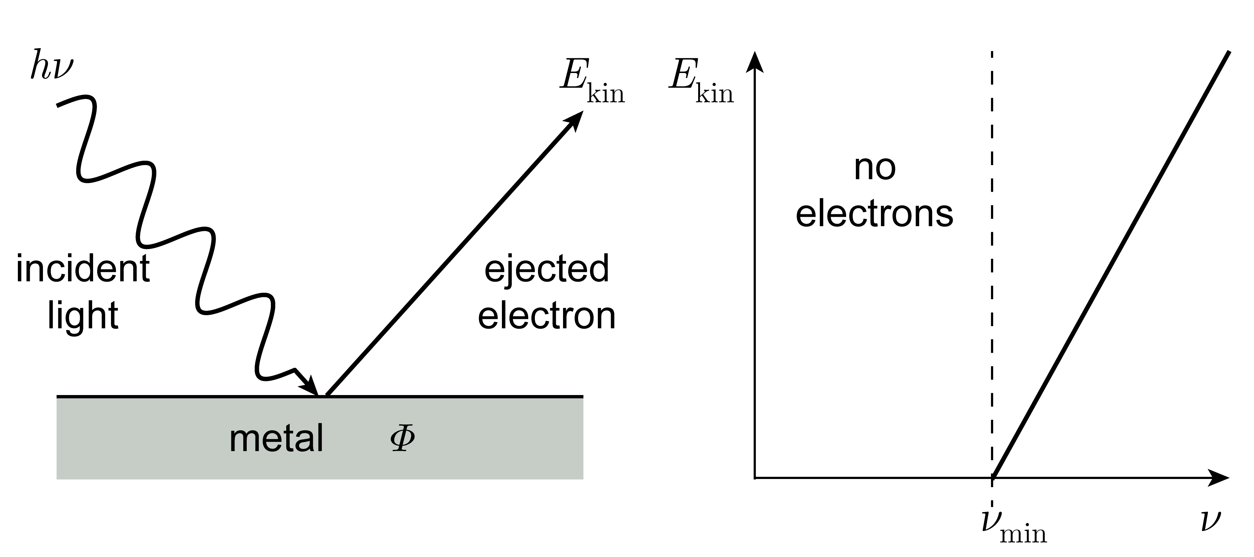
The binding energy of a particle in its ground state in a well of depth \(V_0\) is \(V_0-E_1\). When light with photon energy \(E_\mathrm{ph}\) larger than this is absorbed, the particle is excited to an unbound state - it is ejected from the box. The excess energy is carried away by the particle, that is, it is converted to kinetic energy, \(E_\mathrm{kin}\). The relevant equation is

(3.32)\[E_\mathrm{ph} = \varPhi + E_\mathrm{kin}\]

Example: If 400 nm light hits a Cs surface, electrons are ejection. The incident photon energy is \(E_\mathrm{ph} = hc/\lambda = 3.10\,\mathrm{eV}\). With \(\varPhi = 1.95\,\mathrm{eV}\), the resulting kinetic energy of the ejected electron is \(E_\mathrm{kin} = E_\mathrm{ph} - \varPhi = 1.15\,\mathrm{eV}\). Using \(E_\mathrm{kin} = mv^2/2\), this yields a speed of 636 km/s.

The binding energy of an electron in an isolated molecule is called the ionization energy, \(IE\), and the associated process is called photo-ionization. The same energy for a bulk material (such as a metal) is called the work function, usually indicated by \(\varPhi\). Typical values range from 1.95 eV (Cs) to 5.1 eV (Au).

The emission of electrons from a surface upon irradiation with light of sufficiently high frequency (short wavelength) is called the photoelectric effect. Einstein received his Nobel prize for explaining this effect.

The practical application of the photoelectric effect is called photoelectron spectroscopy or photoemission spectroscopy (PES). It is used to analyze the chemical composition of the surface of solids. It comes in two variants: UPS utilizes UV radiation and extracts valence electrons, whereas XPS uses X-rays and extracts core electrons.

3.5. Free particles

Let us consider the case of a particle freely moving in one dimension, unconstrained by any potential barriers.

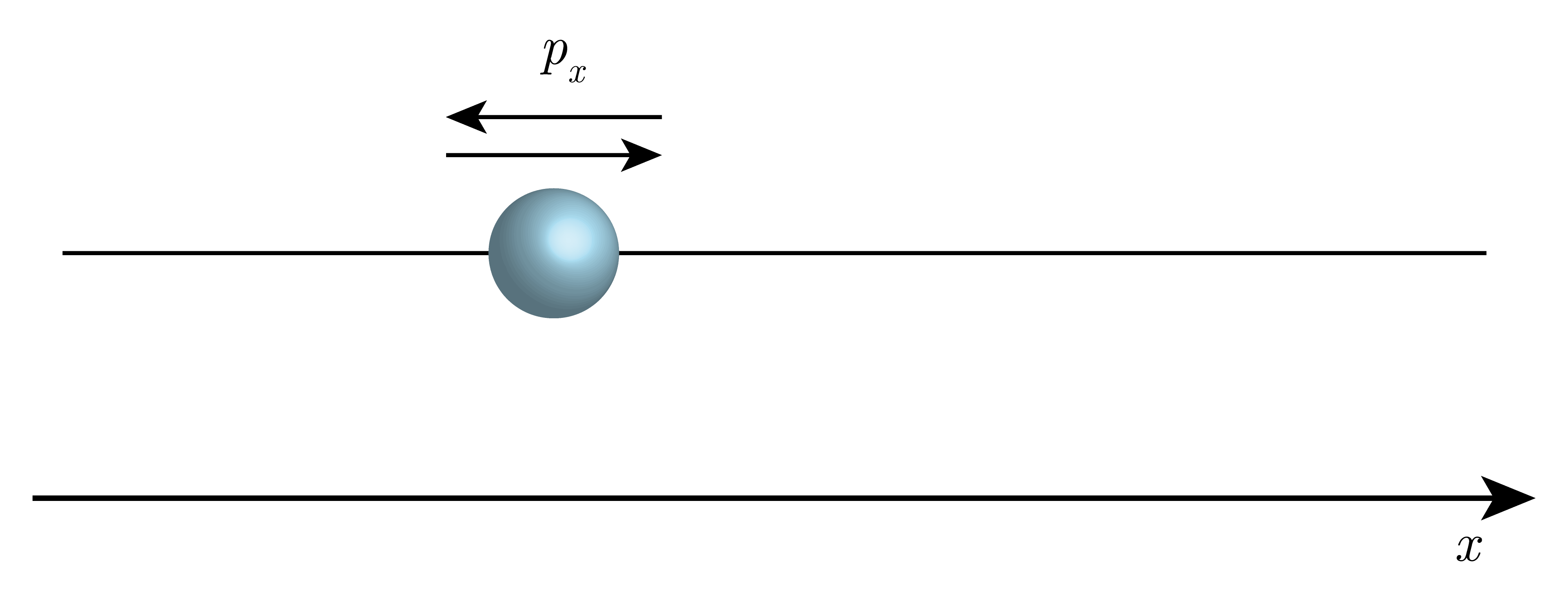
Figure 3.17 A particle free to move along one dimension without any barriers. \(p_x\) indicated the linear momentum of the particle along \(x\).

The Schrödinger equation for this free particle is

(3.33)\[\frac{\mathrm{d}^2}{\mathrm{d} x^2}\psi(x) = -\frac{2mE}{\hbar^2}\cdot\psi(x) = -k^2\cdot \psi(x)\]

where we introduced the abbreviation \(k = \sqrt{2mE}/\hbar\). The general mathematical solution is

(3.34)\[\psi(x) = A\mathrm{e}^{\mathrm{i}kx} + B\mathrm{e}^{-\mathrm{i}kx}\]

with arbitrary constant \(A\) and \(B\). These wavefunctions represent extended plane waves. They are eigenfunctions of the momentum operator:

(3.35)\[\hat{p}_x \mathrm{e}^{\pm\mathrm{i}kx} = -\mathrm{i}\hbar \frac{\mathrm{d}}{\mathrm{d}x} \mathrm{e}^{\pm\mathrm{i}kx} = (\pm\hbar k)\cdot \mathrm{e}^{\pm\mathrm{i}kx}\]

The functions with \(+k\) indicate motion to the right, and those with \(-k\) correspond to motion to the left. \(k\) has dimension of inverse length.

The unknowns in the above wavefunctions are \(A\), \(B\), and \(E\) (through \(k\)). There are no boundary conditions, so there are no constraints on \(E\). In other words, the particle can have any energy!

Additionally, the wavefunctions above are not normalizable! For example, for the function with \(B=0\)

(3.36)\[\int_{-\infty}^\infty \psi^*\psi\,\mathrm{d}x = |A|^2 \int_{-\infty}^\infty \mathrm{e}^{-\mathrm{i}kx}\mathrm{e}^{+\mathrm{i}kx}\,\mathrm{d}x = |A|^2 \int_{-\infty}^\infty \,\mathrm{d}x = \infty\]

We can see why the normalization doesn’t work: Any normalizable function must converge to zero as \(x\rightarrow\pm\infty\). However, this function just keeps oscillating with \(x\).

The fact that \(\psi\) cannot be normalized means that \(\psi\) does not represent a physically possible state, even though it mathemtically solves the time-independent Schrödinger equation.

However, a free particle can be in a non-stationary states that is more localized. The wavefunctions for such a state can be constructed as a superposition of many elementary plane-wave functions with different \(k\):

(3.37)\[\psi(x) = \frac{1}{\sqrt{2\pi}} \int_{-\infty}^\infty \phi(k) \mathrm{e}^{\mathrm{i}kx} \,\mathrm{d}k\]

Here, \(\phi(k)\) represents a distribution of \(k\) values, and the integral integrates the plane waves \(\mathrm{e}^{\mathrm{i}kx\) over this distribution. The resulting superposition wavefunction is more localized, and it decays to zero as \(x\) approaches \(\pm\infty\). Wavefunctions of this form are called wavepackets. Figure 3.18 shows an example.

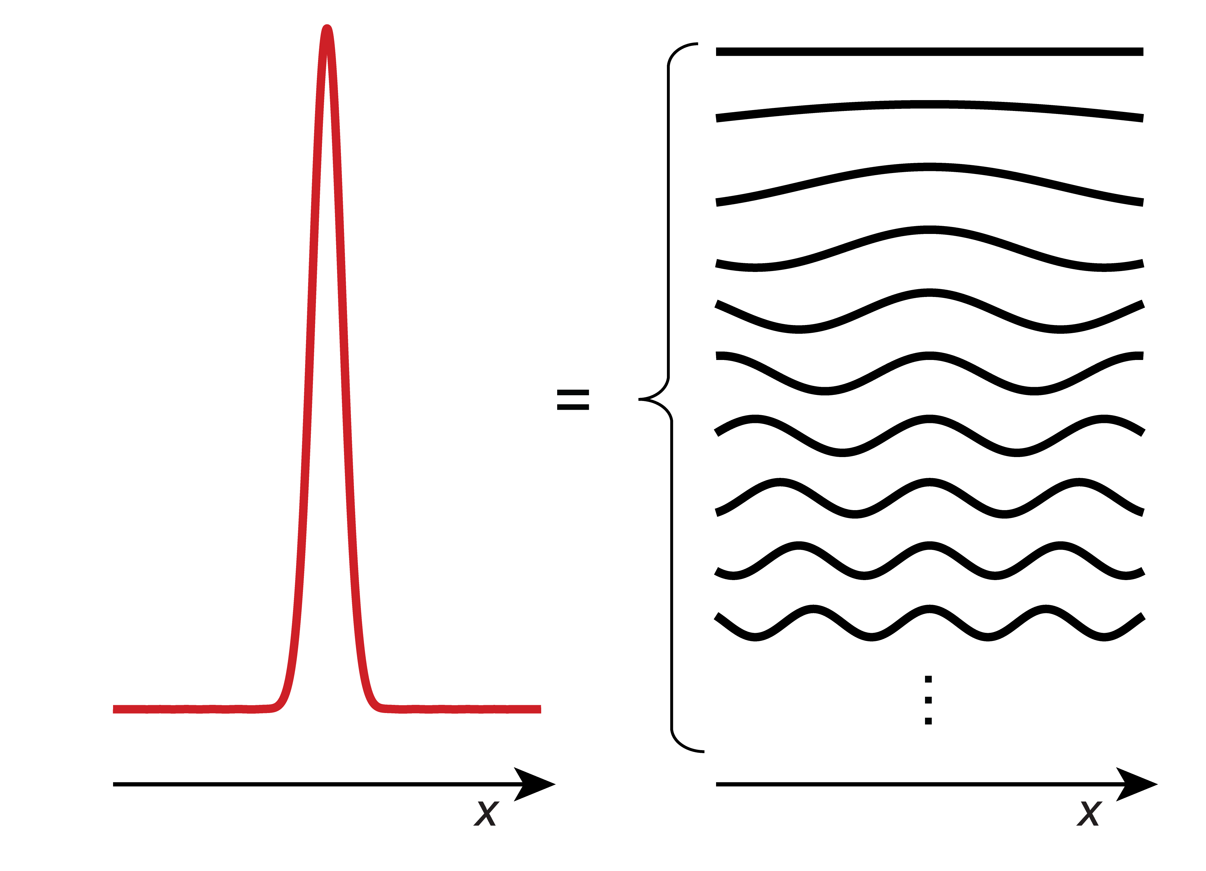
Figure 3.18 A wavepacket is a spatially localized wavefunction. It can be represented as a superposition of extended waves of the form \(\mathrm{e}^{\mathrm{i}kx}\).

The states described by these wavepackets are non-stationary. The wavepackets spread out over time, meaning that the uncertainty about the position of the particle increases as time passes. Also, wavepackets move, similar to actual particles.

The energy relates to \(k\) via \(k=\sqrt{2mE}/\hbar\). Since the wavepacket \(\psi(x)\) is an integral over a range of \(k\), \(psi(k)\) does not have a single defined energy, but rather a distribution.

3.6. Tunneling

Next, we look at the opposite of a potential well: a potential barrier. Figure 3.19 illustrates the potential energy profile for barrier of width \(a\) and height \(V_0\).

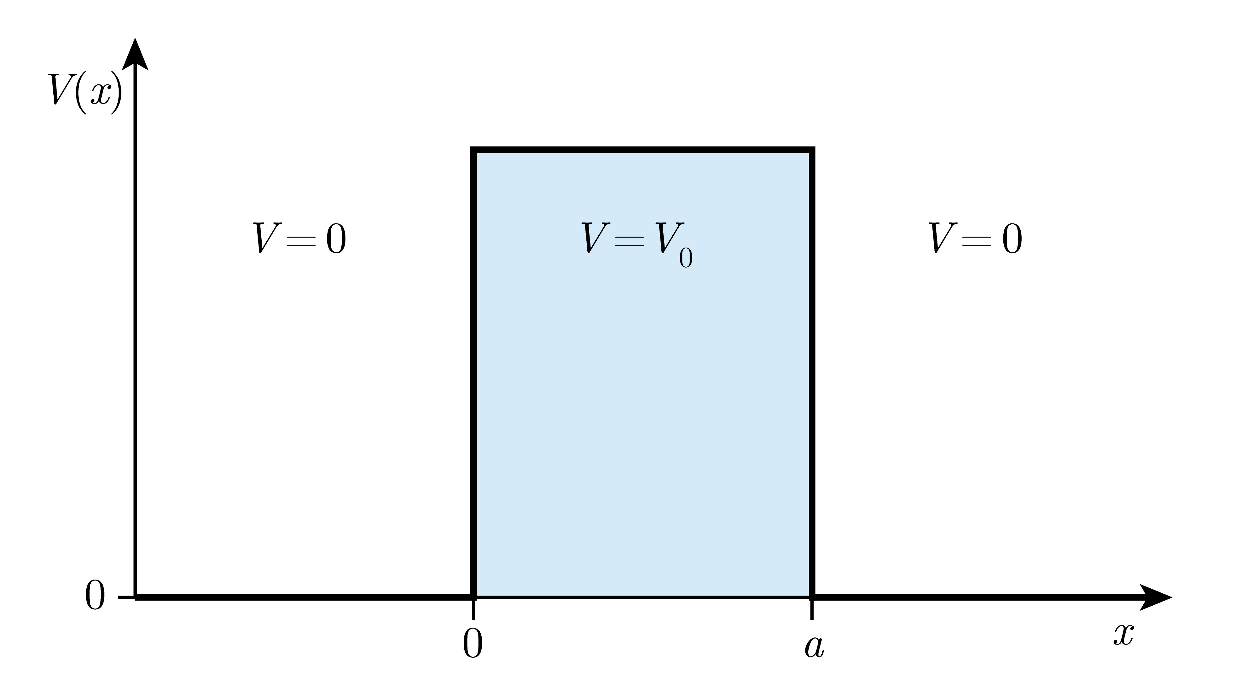
Figure 3.19 A one-dimensional potential-energy barrier.

The transmission probability \(T\) of a particle with mass \(m\) and energy \(E\) across the barrier is

()\[T = \frac{1}{1+q^2\sinh^2(Ka)} \qquad q^2 = \frac{V_0^2}{4E(V_0-E)} \qquad K = \frac{\sqrt{2m(V_0-E)}}{\hbar}\]

where \(\mathrm{sinh}\) is the hyperbolic sine function, defined as \(\mathrm{sinh}(x) = (\mathrm{e}^x-\mathrm{e}^{-x})/2\). This function is plotted in Figure 3.20 (blue curve). If the energy of the particle is near zero, the tunneling probability is near zero. As the energy increases, the probability increases. When the particle energy matches the potential barrier, the transmission probability has not yet reached 100%. It continues to increase monotonically as the energy becomes larger than \(V_0\), until it eventually reaches 100%. However, as the energy increases further, \(T\) drops slightly again. Classically, one predicts the following (see red curve): The particle should not be able to get across the barrier at all as long as \(E<V_0\), and it makes it across with a 100% probability if \(E>V_0\) . The quantum behavior is very different.

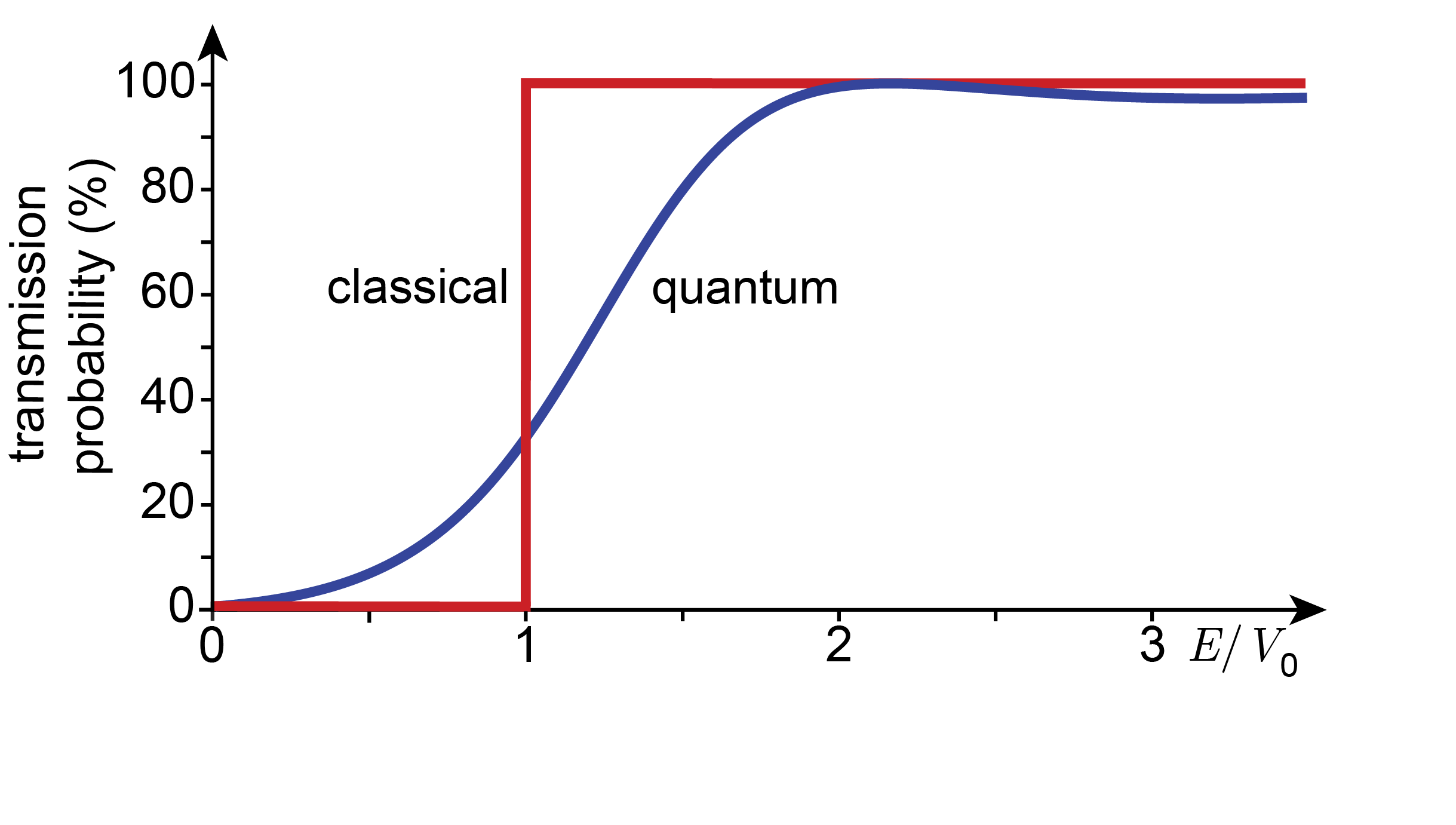
Figure 3.20 Transmission probability for an electron with energy \(E\) across a barrier of 0.4 nm width and 2 eV height.

Tunneling is a phenomenon that is very important in chemistry. \(T\) is strongly dependent on the particle mass \(m\). Lighter particles have larger tunneling probabilities than heavier ones. The two particles that exhibit significant tunneling behavior are electrons and protons. Tunneling is involved in all redox reactions, and it is important for proton transfer reactions as well.

Note

Kinetic isotope effect. In a reaction that involves the transfer of hydrogen from one site to another (for example, from one molecule to another), the kinetics of the transfer will strongly depend on the hydrogen isotope. If \(^1\)H (protium) is replaced by \(^2\)H (deuterium), then the observed reaction rate can slow down significantly if the transfer is via tunneling. The mass of \(^2\)H is twice the mass of \(1\)H, and the tunneling probability \(T\) decreases, reducing the reaction rate. This effect is called the kinetic isotope effect (KIE). This is the main reason why \(^2\)H\(_2\)O (heavy water) would be very toxic - it would disrupt the delicate balance of reaction rates of enzymatic reactions in our bodies. Bacteria that grow well in normal water grow only very slowly, if at all, in heavy water.

Note

The scanning tunneling microscope is an application of tunneling.