4. Molecular vibrations

4.1. Introduction

Chemical bonds between atoms are not perfectly stiff. With sufficient force, they can be stretched or compressed, and they can oscillate, or vibrate, with a frequency that is characteristic of the type of the bond and the atoms connected by it. These molecular vibrations are important in several respects: (1) They are responsible for storing and releasing thermal energy. (2) The vibrational frequencies can be measured using infrared (IR) spectroscopy or Raman spectroscopy and reveal the nature of the chemical bonds in a molecule, providing evidence for identifying its chemical structure.

A chemical bond behaves similar to a mechanical coil spring connecting two point masses. We can characterize the state of such a spring by its length \(r\). At equilibrium, when the spring is neither stretched nor compressed, the length is called the equilibrium length and indicated as \(r_\mathrm{e}\), and \(r\) can be shorter, equal, or longer than \(r_\mathrm{e}\). This is more directly captured by a related quantity, the displacement \(x\), which corresponds to the deviation of the bond length from its equilibrium value:

(4.1)\[x = r - r_\mathrm{e}\]

For a stretched bond, the displacement is positive. For a compressed bond, it is negative. At equilibrium, the displacement is zero (see Figure 4.1).

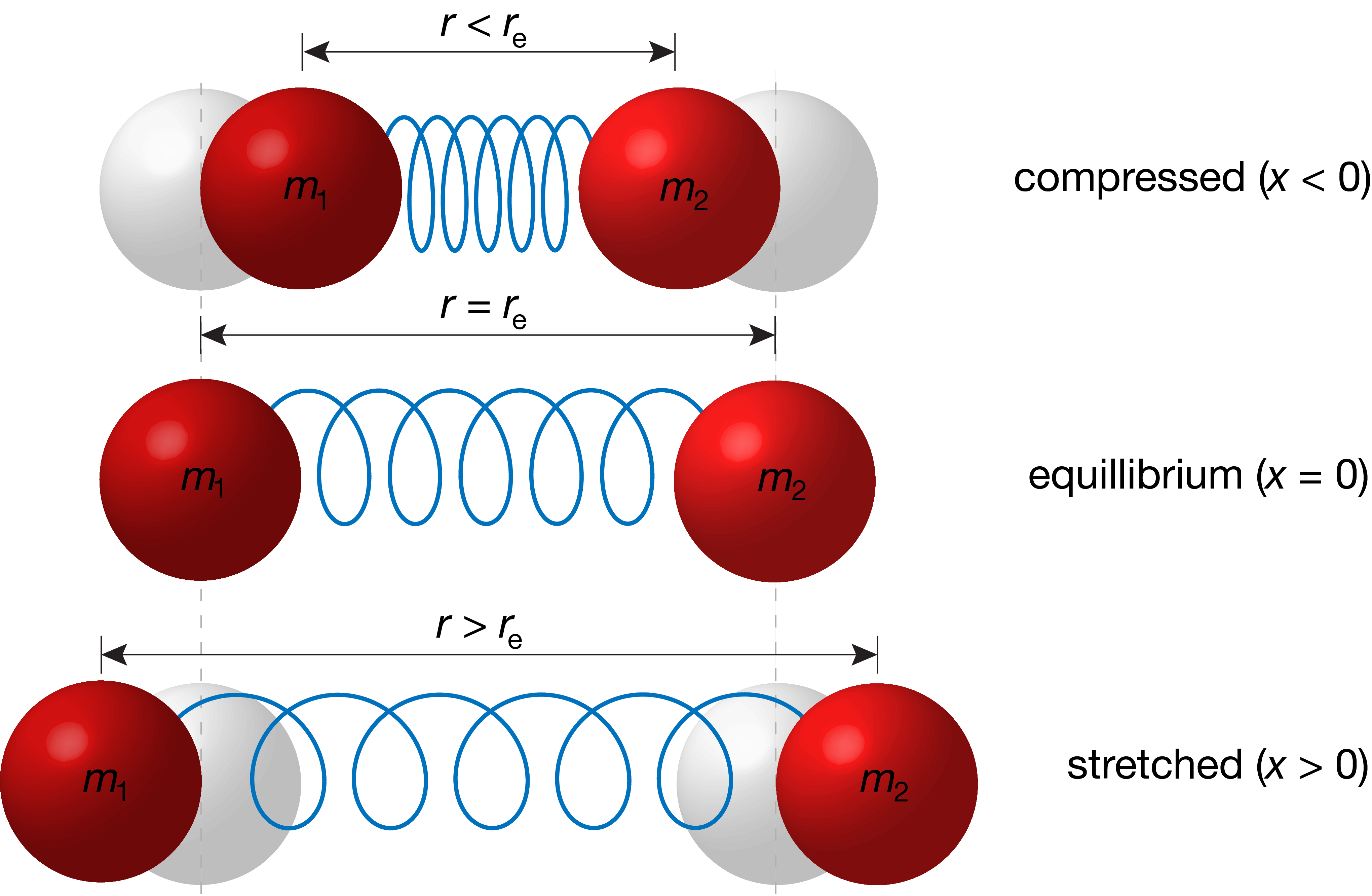
Figure 4.1 Bond length \(r\), equilibrium bond length \(r_\mathrm{e}\), and displacement \(x\) of a chemical bond.

Note

Displacement. The equilbrium bond length of the C-O bond in carbon dioxide, CO\(_2\), is 116 pm. If the bond is stretched to 120 pm, then the displacement is +4 pm. If the bond is compressed to 114 pm, the displacement is -2 pm.

The simplest model of a idealized spring follows Hooke’s law: When stretched or compressed, it experiences a restoring force \(F\) that pushes the spring back towards the equilibrium (zero displacement), and this force is proportional to the displacement: \(F = -k(r-r_\mathrm{e}) = -k x\). The proportionality constant \(k\) is called the force constant and has SI units of N/m (newtons per meter). A large value of the force constant indicates a stiff bond that is hard to stretch or compress, and a small value indicates a loose bond that is easily deformed. The potential energy associated with this force is a quadratic function of the displacement:

(4.2)\[V(r) = \frac{1}{2}k (r-r_\mathrm{e})^2 = \frac{1}{2}k x^2\]

This indicates that there is a minimum of the potential energy at the equilibrium bond length, and that it grows quadratically as the bond length is shortened or lengthened.

A bond or spring that has a perfectly quadratic potential is called a harmonic oscillator. However, this is never the case in the real world of chemical bonds. A more realistic potential-energy curve is shown in Figure 4.2. It differs from the harmonic oscillator in two respects: (1) When a bond is stretched, it will eventually break, and once broken, the potential energy will be independent of the inter-atomic distance and there will be no restoring force. This is indicated by the fact that \(V(r)\) converges and goes flat as \(r\) increases. (2) when a bond is compressed, it becomes rapidly very hard to compress it further, as the electrons in the core orbitals of the two atoms repel each other strongly. This is reflected in the potential-energy curve \(V(r)\) by a rapid growth as the bond length is shortened, more rapid than the harmonic potential.

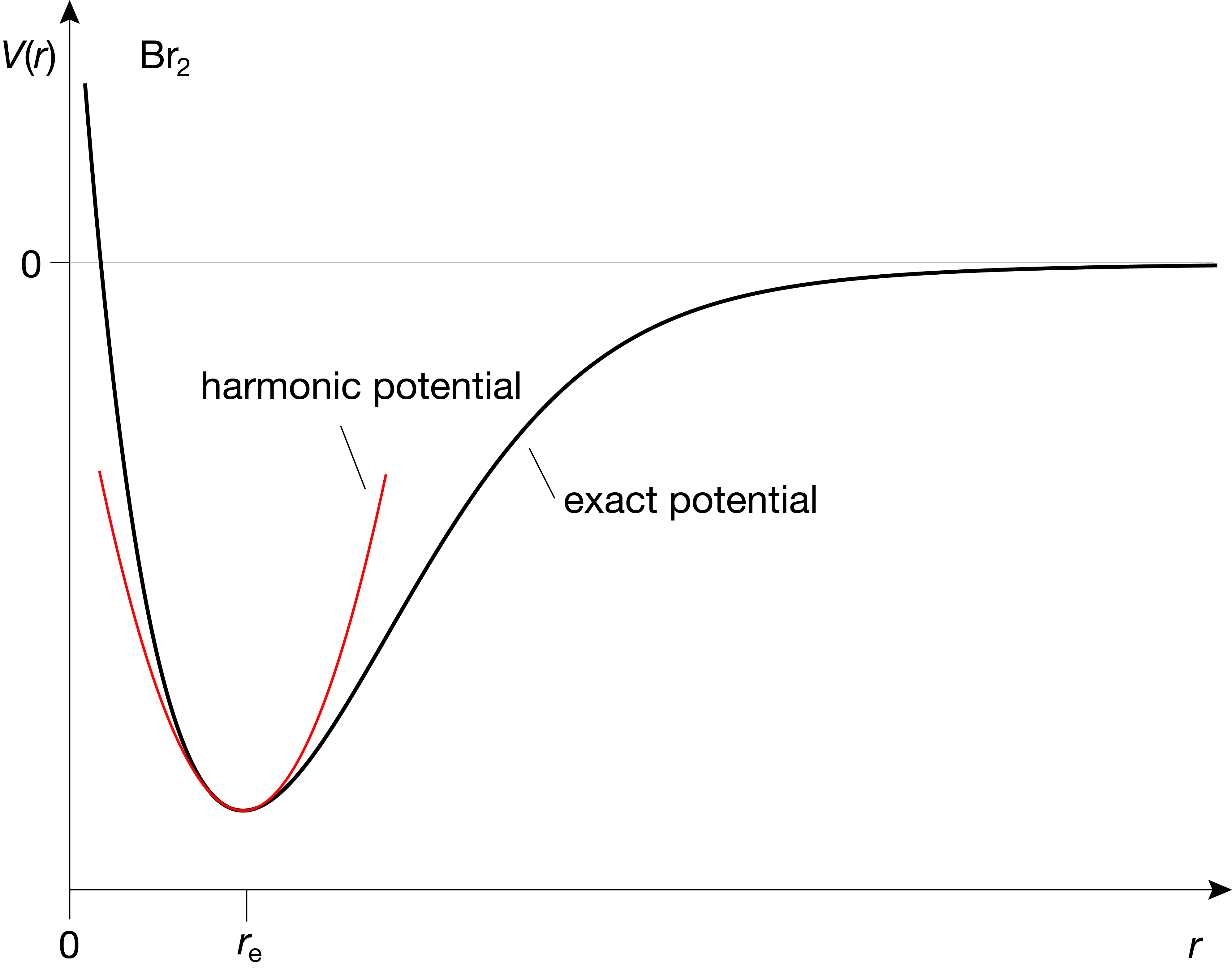
Figure 4.2 Comparison between a real-world inter-atomic potential and the harmonic potential.

Despite the differences to real-world potentials, the quadratic potential is a good approximation near the equilibrium length (around zero displacement), which is the region where most bonds are found at room temperature. Therefore, the theory of molecular vibrations is based on the harmonic potential. Deviations from the harmonic model are called anharmonicity and are treated as corrections.

Note

We can write the potential-energy function near the equilibrium distance in the form of a Taylor series, with terms containing derivatives of increasing order:

(4.3)\[V(r) = V(r_\mathrm{e}) + \frac{\partial V(r)}{\partial r}{\Big|}_{r = r_\mathrm{e}} (r-r_\mathrm{e}) + \frac{1}{2} \frac{\partial^2 V(r)}{\partial r^2}{\Big|}_{r = r_\mathrm{e}} (r-r_\mathrm{e})^2 + \cdots \qquad\]

where the dots indicate terms with third- and higher-order derivatives. The first term (\(V(r_\mathrm{e})=-D_\mathrm{e}\)) shifts all energies by the same amount and does not affect any observed transitions. We can therefore drop it. The second term, containing the first derivative, is zero, since we are at a minimum. Therefore, this drops out as well. The first non-zero term is the third one, with the second derivative. Neglecting all higher-order terms, we can approximate the potential near the equilibrium geometry as

(4.4)\[V(r) \approx \frac{1}{2}k (r-r_\mathrm{e})^2 \qquad \text{with} \qquad k = \frac{\partial^2 V(r)}{\partial r^2}{\Big|}_{r = r_\mathrm{e}}\]

This shows that the force constant is the second derivative of the potential energy at the equilibrium bond length.

4.2. Classical harmonic oscillator

We start with the simplest type of molecules that can vibrate: diatomic molecules. For the purpose of modeling its vibration, a diatomic molecule can be considered as consisting of two masses \(m_1\) and \(m_2\) connected by a massless spring with spring constant \(k\).

In order to determine the energies and wavefunctions associated with the vibrational motion along the displacement coordinate, we first have to separate this motion from all other types of motion of the molecule. Since each atom can move in three mutually perpendicular directions, it has three degrees of freedom. With two atoms, this gives a total of six degrees of freedom. We are not interested in the overall motion of the molecule: translation (3 degrees of freedom: left/right, top/bottom, front/back) or rotation (2 degrees of freedom: around vertical axis, around axis perpendicular to the screen/paper). This leaves one degree of freedom that is internal, the bond length.

In order to calculate the vibration frequency for the bond, this two-particle problem is reduced to an effective one-particle problem. In this procedure (see derivation), the center-of-mass is separated out, and the two atoms with masses \(m_1\) and \(m_2\) are replaced by a single pseudo-particle with the so-called reduced mass \(\mu\):

(4.5)\[\mu = \frac{m_1m_2}{m_1+m_2}\]

Note

For atoms and molecules, \(\mu\) is usually given in atomic mass units, u. The reduced mass is always smaller than the smaller of the two masses. For example, hydrogen fluoride HF with \(m_1\approx 1\,\mathrm{u}\) and \(m_2\approx 19\,\mathrm{u}\) has a reduced mass of approximately \(1\,\mathrm{u}\cdot 19\,\mathrm{u}/(1\,\mathrm{u}+19\,\mathrm{u}) \approx 0.95\,\mathrm{u}\). This is smaller than 1 u.

Figure 4.3 illustrates schematically the transformation from a two-particle to a one-particle system.

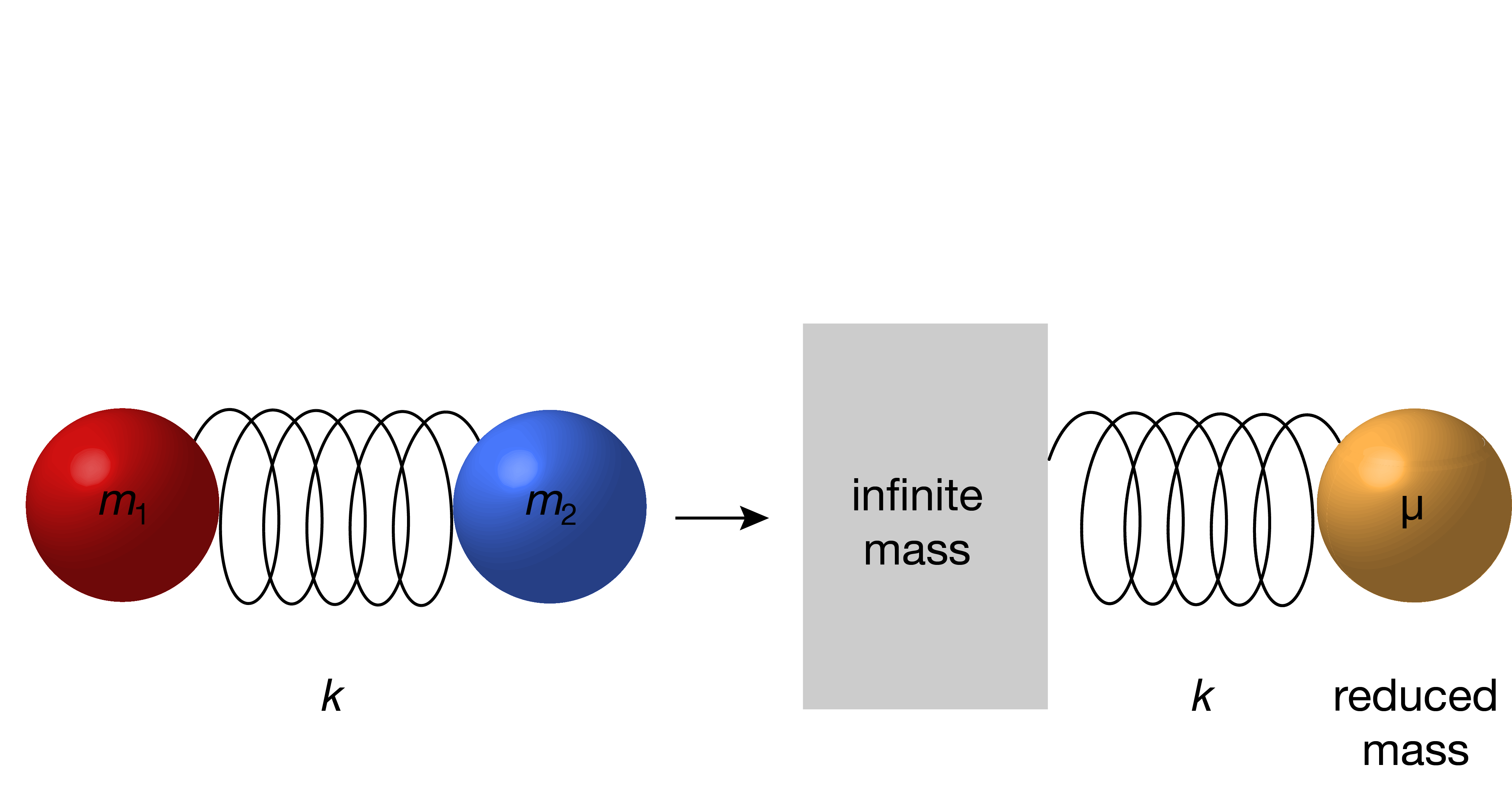
Figure 4.3 Transformation from a two-particle system with masses \(m_1\) and \(m_2\) to a one-particle system with the reduced mass \(\mu\).

In this one-particle formulation, it is now possible to calculate the oscillator frequency, which is

(4.6)\[\omega_\mathrm{e} = 2\pi\nu_\mathrm{e} = 2\pi c{\tilde\nu}_\mathrm{e} = \sqrt{\frac{k}{\mu}}\]

Here, \(\omega_\mathrm{e}\) is the angular frequency (in radians per second), \(\nu_\mathrm{e}\) is the ordinary frequency (in hertz = cycles per second), and \(\tilde\nu_\mathrm{e}\) is the wavenumber (in inverse centimeters, cm^-1). This equation reveals that the oscillator frequency increases with increasing force constant, but decreases with increasing mass. Therefore, loose bonds in heavy molecules have slow oscillations, and stiff bonds in light molecules have fast oscillations.

Note

The reduced mass of hydrogen fluoride, ¹H¹⁹F, is 0.95 u, and the force constant of the bond is 959 N/m. This gives an oscillator frequency of 124 THz (terahertz), with a period of about 8 fs (femtoseconds). The corresponding wavenumber is 4138 cm^-1.

We can rearrange this equation to express the force constant in terms of the reduced mass and the oscillator frequency:

(4.7)\[k = \mu \omega_\mathrm{e}^2 = \mu \left(2\pi c{\tilde\nu}_\mathrm{e}\right)^2\]

4.3. Quantum harmonic oscillator

The Hamiltonian for the quantum harmonic oscillator combines the kinetic-energy operator and the quadratic potential-energy term

(4.8)\[\hat{H} = -\frac{\hbar^2}{2\mu}\frac{\mathrm{d}^2}{\mathrm{d}x^2} + \frac{1}{2}k x^2 = -\frac{\hbar^2}{2\mu}\frac{\mathrm{d}^2}{\mathrm{d}x^2} + \frac{1}{2}\mu\omega_\mathrm{e}^2 x^2\]

Solving the time-independent Schrödinger equation \(\hat{H}\psi(x) = E\psi(x)\) with this Hamiltonian yields energies and wavefunctions for the stationary states (see derivation). As for the particle-in-the-box model, one obtains an infinite number of mathematically correct solutions. All these solutions solve the time-independent Schrödinger equation, but most of the solutions for \(\psi\) are non-physical, since they diverge for \(x\rightarrow\pm\infty\) and therefore are not normalizable. Only a small subset of the solutions, indicated by \(\psi_n(x)\) (with the integer index \(n=0,1,2,\dots\)) are normalizable. These have the associated energies:

(4.9)\[E_n = \hbar\omega_\mathrm{e} \left(n+\frac{1}{2}\right) = hc\tilde\nu_\mathrm{e} \left(n+\frac{1}{2}\right) \qquad\qquad n=0,1,2,\dots\]

where \(n\) is the vibrational quantum number (sometimes indicated by the Greek letter upsilon, \(\upsilon\), that must be distinguished carefully from the Greek letter nu, \(\nu\), and from the Latin letter vee, v). All states are non-degenerate, that is, for each energy \(E_n\), there is only one state. Note also that we have a single degree of freedom (the displacement) and therefore one quantum number - this is another instance of the rule that there is one quantum number per (constrained) degree of freedom.

Let’s revisit what this means. A harmonic oscillator can be in any of a series of stationary states, each of them labeled with the quantum number \(n\) and described by the wavefunction \(\psi_n(x)\). Each of these states has a defined energy, given by \(E_n\). The harmonic oscillator can only assume stationary states with certain energies, and not others. This is meant when we say that the energy is quantized.

Regarding the energy levels, we can make three observations: (a) The energies are quantized. As stated, this is a consequence of the requirement that the associated wavefunctions are normalizable. (b) The energies are evenly spaced - two adjacent levels \(n\) and \(n+1\) are separated by \(\hbar\omega_\mathrm{e}\), no matter what the value of \(n\) is. (c) The ground state (\(n =0\)) has a non-zero energy, just like the particle-in-a-box. This zero-point energy indicates that there is some residual kinetic energy and motion that cannot be removed from the system since it is already in its lowest-energy state.

Note

Relevance of zero-point energy. The zero-point energy (ZPE) of a molecule becomes relevant in chemical reactions, where bonds are broken and formed. If a bond is broken, the ZPE is released.

Figure 4.4 illustrates the vibrational energy level diagram for a diatomic molecule with a stiff bond (nitrogen N₂; left) and one with a looser bond (fluorine F₂; right). The difference is mostly due to the difference in force constants (a factor of 5), and not from the difference in reduced mass (9.5 u vs. 7 u).

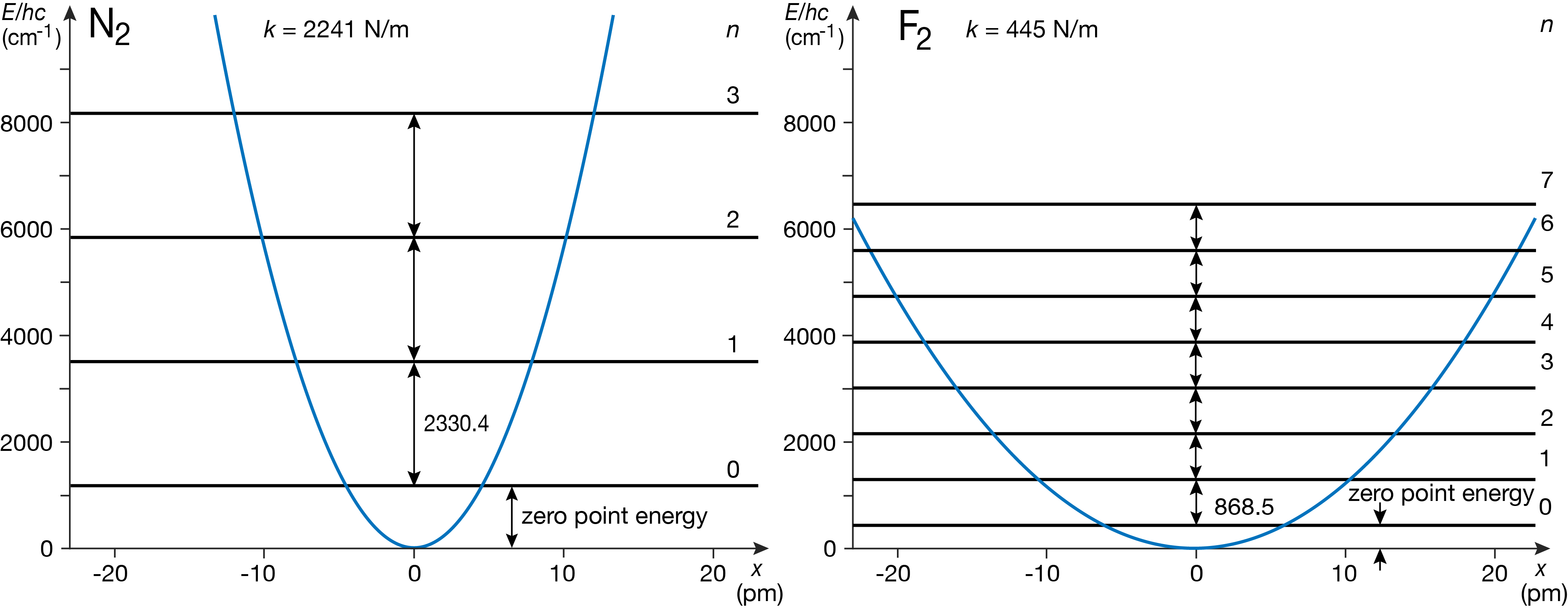
Figure 4.4 Effect of force constant and reduced mass on vibrational energy levels.

4.4. Wavefunctions

The general expression for the wavefunctions for the stationary states of the harmonic oscillator are

(4.10)\[\psi_n(x) = N_n\cdot H_n(x\sqrt{\alpha})\cdot\mathrm{e}^{-\alpha x^2/2}\]

with \(\alpha = \mu\omega_\mathrm{e}/\hbar = \sqrt{\mu k}/\hbar\) and the normalization constant \(N_n=(\alpha/\pi)^{1/4}/\sqrt{2^nn!}\). The functions \(H_n(\cdot)\) are called Hermite polynomials (see Appendix). The Hermite polynomials are oscillatory, and they go to \(\pm\)infinity as \(x\) moves away from zero. The last factor is a Gaussian function and is always positive. It is maximal at \(x = 0\) and converges towards zero as \(x\) moves away from that. The exponential of the Gaussian function, however, shrinks faster than the polynomial grows and therefore guarantees that the overall wavefunction tapers down to zero on both sides and is normalizable and physical.

The specific wavefunctions for the ground state (\(n=0\)) and the first excited state (\(n=1\)) are

(4.11)\[\begin{split}\begin{align} \psi_0(x) &= \left(\frac{\alpha}{\pi}\right)^{1/4}\cdot\mathrm{e}^{-\alpha x^2/2}\\ \psi_1(x) &= \frac{1}{\sqrt{2}}\left(\frac{\alpha}{\pi}\right)^{1/4}\cdot2x\sqrt{\alpha}\cdot\mathrm{e}^{-\alpha x^2/2} \end{align}\end{split}\]

Figure 4.5 illustrates the vibrational wavefunctions for the lowest-energy states. The general shape of the wavefunctions is similar to the ones in the particle in the box and in the finite-depth potential well: The ground-state wavefunction has one half-wave, the first excited-state wavefunction has two half-waves, and so on.

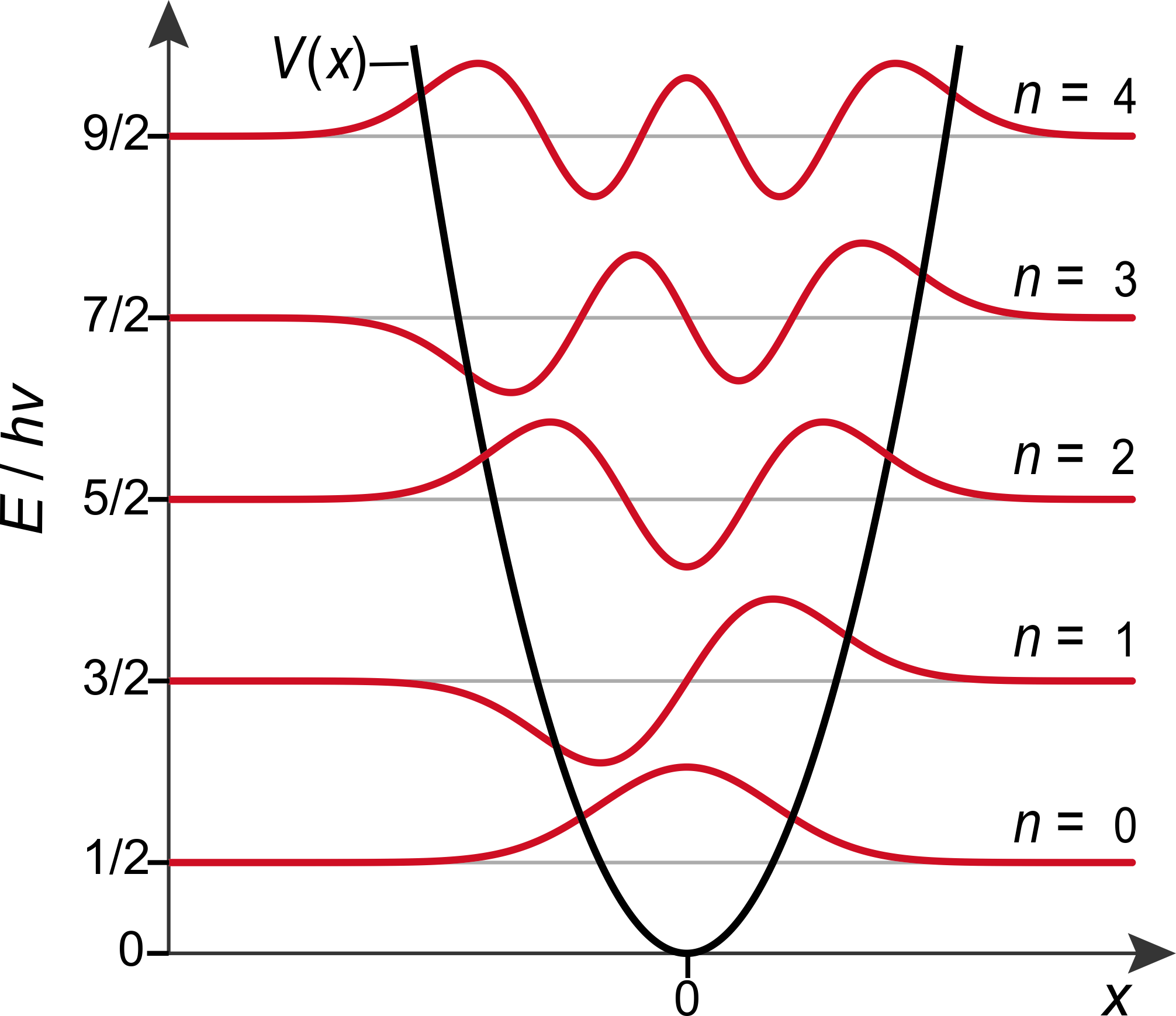
Figure 4.5 The wavefunctions of the harmonic oscillator.

Figure 4.6 shows the associated probability densities. The probability density of the ground state shows that even in this lowest-energy state, the chemical bond length is not sharply defined. It is somewhat “delocalized”, in the sense that repeated measurements on molecules in the ground state will yield slightly different bond lengths, which a distribution corresponding to \(|\psi_0(x)|^2\).

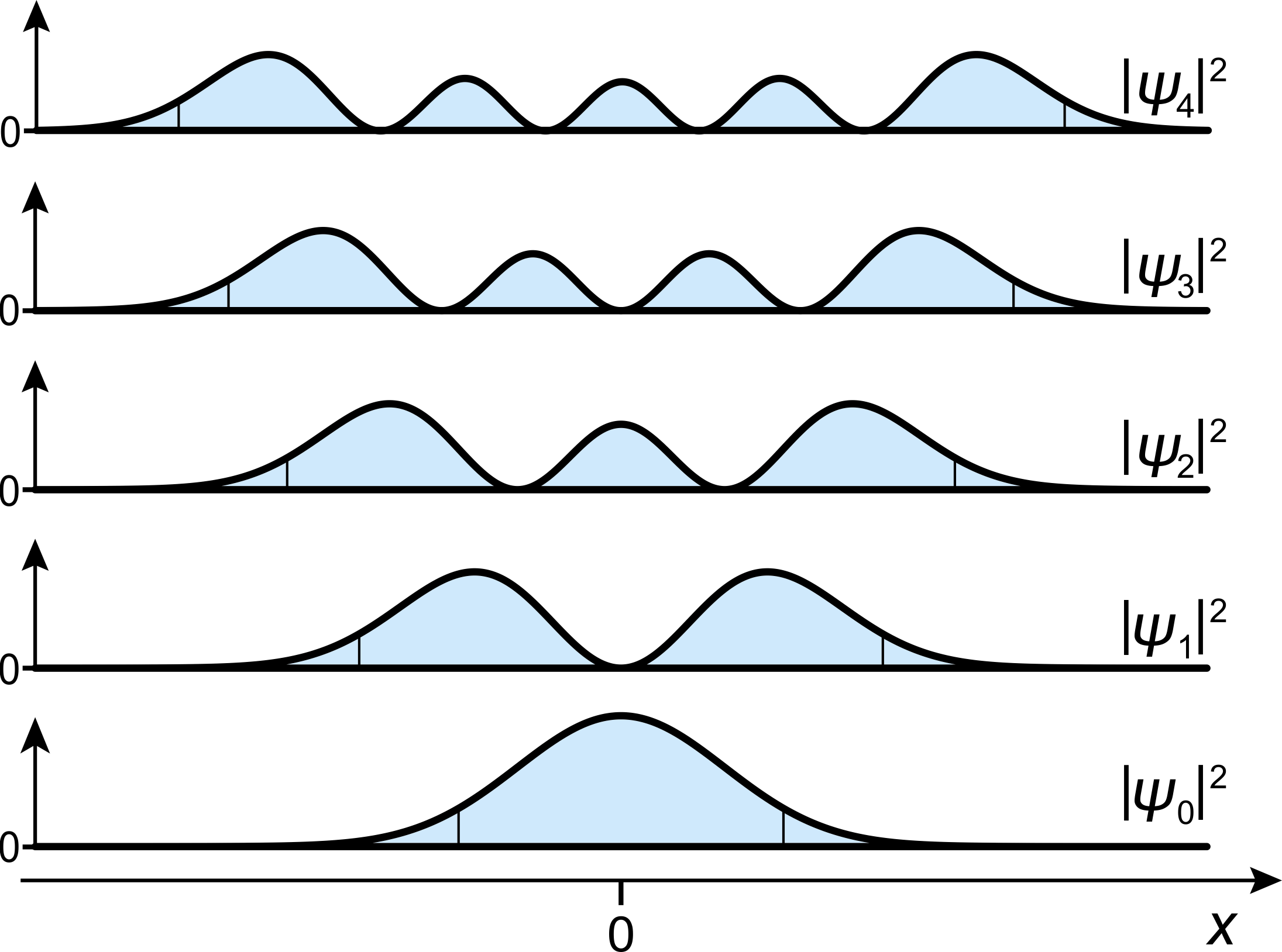
Figure 4.6 The probability densities of the harmonic oscillator. The borders between the central classically allowed region (where \(E_n\ge V(x)\)) and the two flanking classically forbidden regions (where \(E_n<V(x)\)) are indicated with thin vertical lines.

This is illustrated in Figure 4.7. The bond delocalization depends on the reduced mass and on the force constant. The bonds in diatomic molecules containing a hydrogen atom are more delocalized than others.

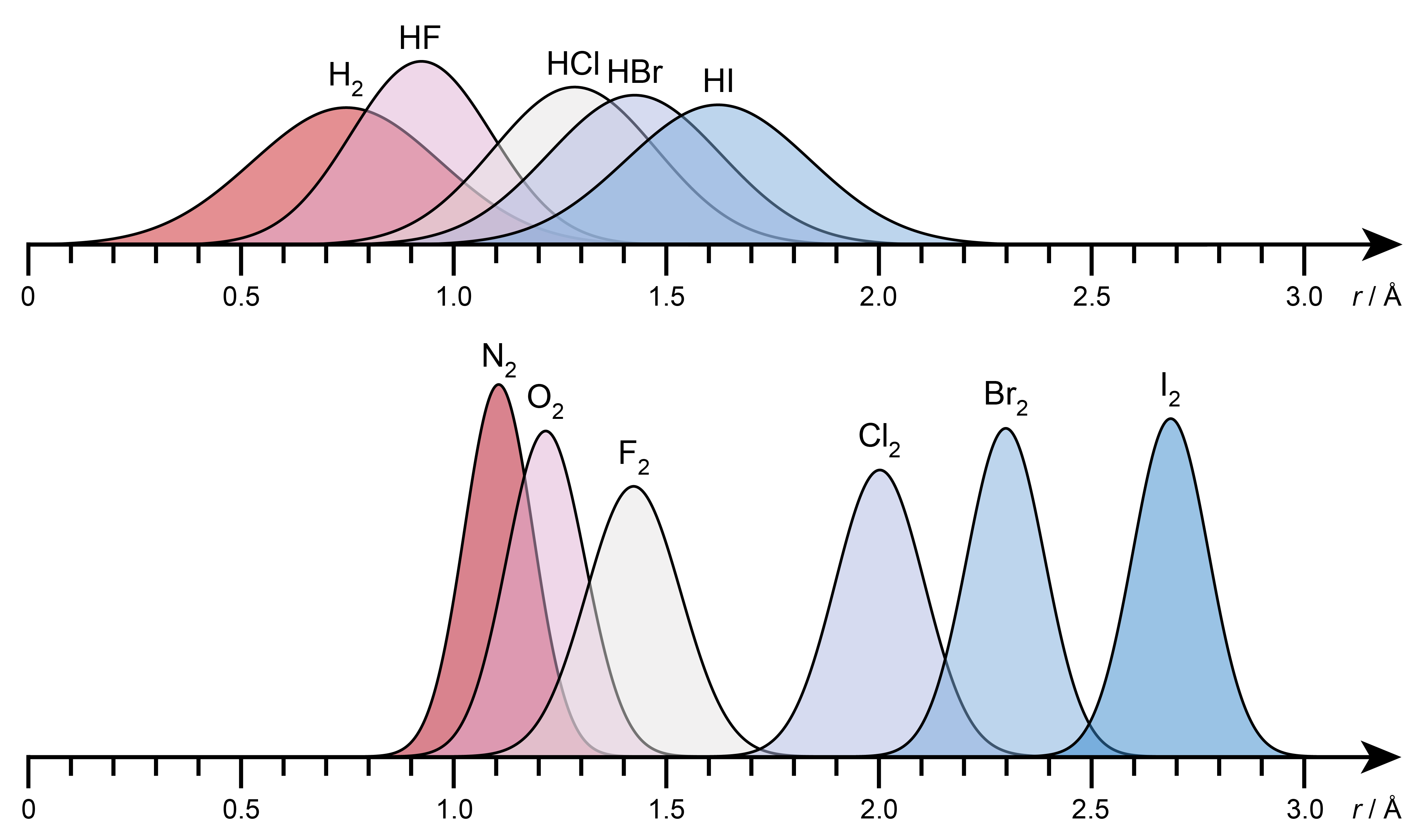
Figure 4.7 The probability densities for the bond lengths for a series of diatomic molecules (top: containing hydrogen, bottom: not containing hydrogen).

4.5. Vibrational transitions

A key quantity in all of spectroscopy is the electric dipole moment \(\boldsymbol{\mu}_\mathrm{el}\) of a molecule. It is the charge-weighted sum of the position vectors of all particles:

(4.12)\[\boldsymbol{\mu}_\mathrm{el} = \sum_k \boldsymbol{r}_k q_k\]

\(\boldsymbol{r}_k\) is the vector indicating the position of particle \(k\), and \(q_k\) is its charge. For molecular vibrations, the particles are atoms and the charges are their partial charges. Figure 4.8 illustrates this.

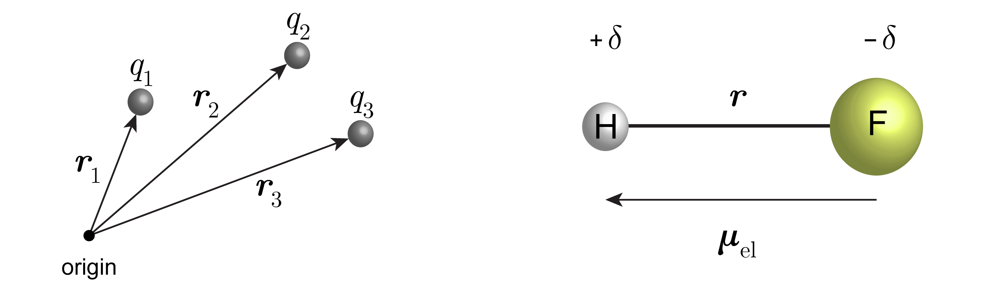
Figure 4.8 The electric dipole moment. Left: the quantities determining the electric dipole moment (positions and charges). Right: Simple case of a neutral diatomic molecule with partial positive and negative charges \(+\delta\) and \(-\delta\) on the two atoms. In this case, the electric dipole moment is \(\delta\cdot\boldsymbol{r}\).

For a neutral diatomic molecule, the electric-dipole moment vector points along the bond, from the more negatively to the more positively charged atom. The SI unit for the electric dipole moment is C m (coulomb-meter), but for molecules it is more convenient to use the conventional unit D (debye), defined as \(1\,\mathrm{D} \approx 3.3356\cdot10^{-30}\,\mathrm{C\,m}\).

Note

To get a sense for the magnitude of electric dipole moments, 1 D corresponds to about 0.21 e Å, where e is the elementary charge. This value corresponds to the situation of two charges of +e and -e separated by 0.21 Å, or two charges of +0.21 e and -0.21 e separated by 1 Å. Diatomic molecules have electric dipole moments of a few D.

The quantum operator for the electric dipole moment is identical to the classical expression, i.e. \(\hat{\boldsymbol{\mu}_\mathrm{el}} = \boldsymbol{\mu}_\mathrm{el}\) - recall that position variables like \(\boldsymbol{r}\) are left unchanged when converting a classical expression to its quantum analog.

When light interacts with a system of quantum particles (electrons and nuclei), the oscillating electric-field component of the radiation interacts with the charged particles by pushing and pulling on the charges. This interaction adds to the total energy of the molecule, and the Hamiltonian gets an additional term

(4.13)\[\hat{H} = \hat{H}_0 - \hat{\boldsymbol{\mu}}_\mathrm{el} \boldsymbol{\mathcal{E}}\]

where \(\boldsymbol{\mathcal{E}}\) is the electric field component of the radiation. The intensity of a transition between two vibrational states with quantum numbers \(n\) and \(n'\) is proportional to the square of the electric transition dipole moment integral:

(4.14)\[\mathrm{intensity} \propto |\langle\psi_{n'}|\hat{\boldsymbol{\mu}}_\mathrm{el}|\psi_n\rangle|^2\]

Evaluating this integral leads to an explicit expression from which a set of necessary conditions can be gleaned which have to be satisfied in order for the transition to happen. These conditions are called selection rules. When they are satisfied, the transition is said to be an allowed transition, otherwise it is a forbidden transition.

The selection rule for transitions for a harmonic oscillator comes in two parts. First, the change in vibrational quantum number from the initial to the final state must be \(\pm 1\) (\(+1\) for absorption and \(-1\) for emission):

(4.15)\[\Delta n = n' - n = \pm 1\]

This means that only transitions between adjacent levels are possible! For these, the energy difference is \(\Delta E = \hbar\omega_\mathrm{e}\), independent of the value of \(n\).

(In reality, the inter-atomic potential energy in molecules is not perfectly harmonic. Therefore, transitions that are fully forbidden according to this selection rule can be weakly allowed.)

Second, molecules must have an electric dipole moment that varies with displacement around the equilibrium position (\(x=0\)), i.e.

(4.16)\[\left.\frac{\mathrm{d}\mu_\mathrm{el}}{\mathrm{d}x}\right|_{x=0}\neq 0\]

This implies that diatomic molecules whose dipole moment doesn’t change with displacement don’t absorb any infrared radiation. This applies particularly to homonuclear diatomic molecules such as N₂, O₂, H₂, etc. In these molecules, vibrational transitions are impossible (forbidden), because the electric-dipole moment is zero at equilibrium and stays zero as the bond is stretched or compressed. On the other hand, heteroatomic molecules such as CO, H₂O, CO₂, CH₄, etc have allowed vibrational transitions and absorb infrared radiation, because their electric dipole moment (zero for CH₄, and non-zero for the others) changes as the molecule vibrates.

Note

Global warming. The most common atmospheric gases are homodiatomic: N₂ and O₂. These do not absorb infrared radiation. On the other hand, other atmospheric gases such as CO₂ and CH₄ are strong absorbers of infrared radiation and therefore are crucial in determining the temperature of the atmosphere - they are greenhouse gases. The dramatic increase in atmospheric CO₂ over the last 1.5 centuries (from below 300 pm to 400 ppm) is the reason for globally rising temperatures.

Note

Atmosphere on Venus. Venus has an atmosphere almost entirely consisting of CO₂ (about 96.5%). As a consequence, the temperature on Venus’ surface is very high, about 700 K.

4.6. Anharmonicity

As discussed in the introduction to this chapter and shown in Figure 4.2, real-world potential-energy functions are not quadratic. Molecular bonds are easier to stretch than a harmonic oscillator (they break eventually), and harder to compress. These deviations from the harmonic-oscillator model are called anharmonicity.

The real-world potential determines the vibrational properties, and they are different from those of an idealized harmonic oscillator: (1) There is only a finite number of vibrational states (\(n=0,1,\dots,n_\mathrm{max}\)); (2) The spacing between adjacent levels is not equal, it decreases with increasing quantum number; (3) The harmonic-oscillator selection rules are not 100% valid: In addition to the allowed fundamental transition between the states \(n=0\) and \(n=1\), overtone transitions \(0\rightarrow 2\), \(0\rightarrow 3\), etc. are observable, although with weak intensities.

The shapes of real-world inter-atomic potentials are derived from experimental data. There exist a few analytical approximative models.

One group of models utilizes exponential functions. Among them, the simplest is the Morse potential, given by the expression

(4.17)\[V_\mathrm{M}(r) = D_\mathrm{e} \left(1 - \mathrm{e}^{-\alpha(r-r_\mathrm{e})} \right)^2 \qquad \alpha = \sqrt{k/2D_\mathrm{e}}\]

where \(D_\mathrm{e}\) is the depth of the potential well, i.e. the difference between \(V(r_\mathrm{e})\) and \(V\) at infinite \(r\). \(r_\mathrm{e}\) is the equilibrium bond length. The Morse potential works very well in approximating real inter-atomic potentials. Figure 4.9 shows the Morse potential in comparison to the harmonic potential.

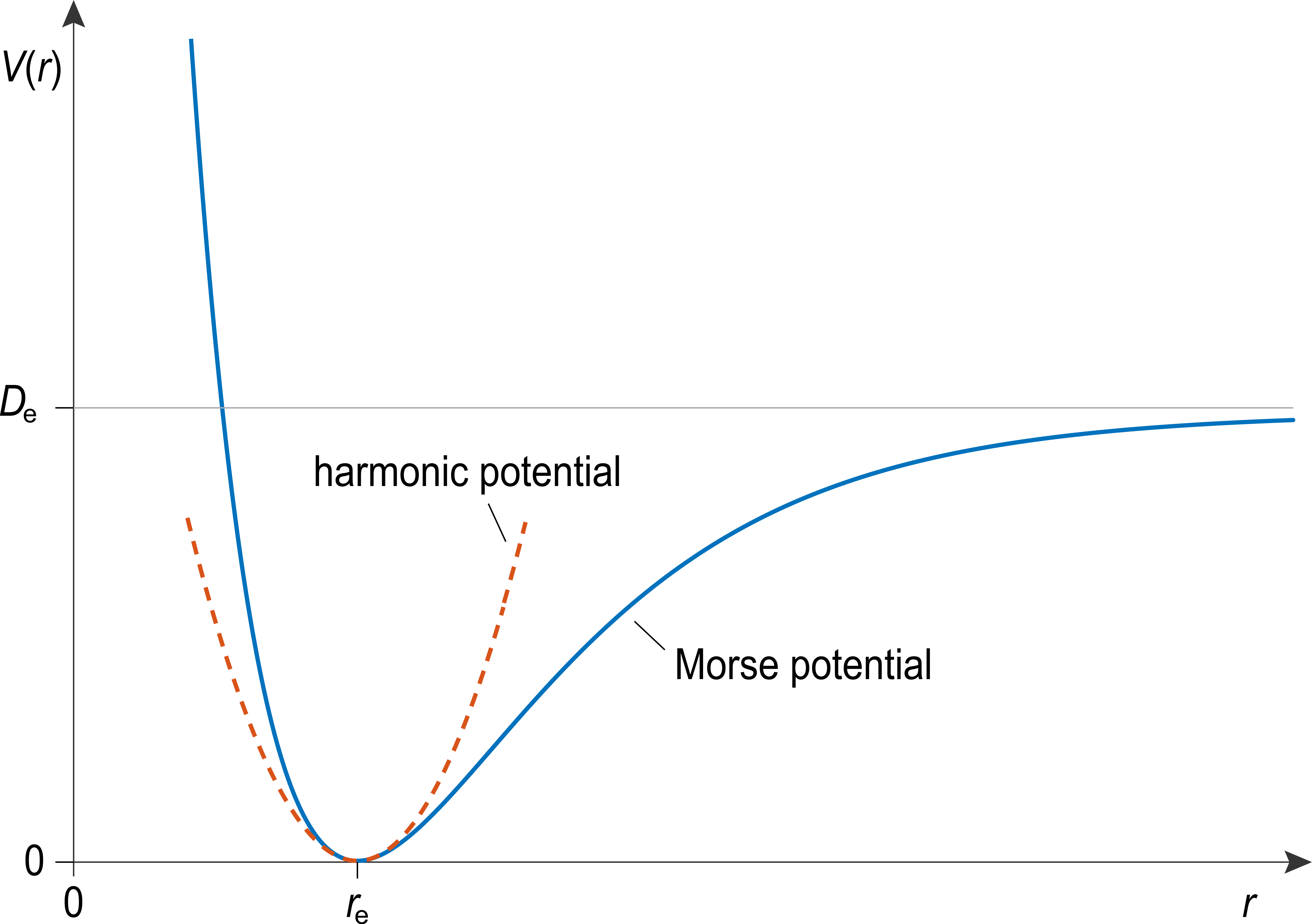
Figure 4.9 The Morse potential.

A nice feature of the Morse potential is that its energy eigenvalues have a closed-form expression:

(4.18)\[E_n = hc\tilde\nu_\mathrm{e} \left(n+\frac{1}{2}\right) - \frac{(hc\tilde\nu_\mathrm{e})^2}{4D_\mathrm{e}} \left(n+\frac{1}{2}\right)^2\]

The first term is identical to the harmonic oscillator. The second term is a correction quadratic both in \(n\) and in \(\tilde\nu_\mathrm{e}\). The prefactor in this term is commonly written as \(hc\tilde\nu_\mathrm{e}x_\mathrm{e}\), with \(x_\mathrm{e} = hc\tilde\nu_\mathrm{e}/(4D_\mathrm{e})\).

A second group of analytical expressions that are often used to approximate real-world potentials uses an expansion in terms of inverse powers of \(r\). The most common of these is the Lennard-Jones potential:

(4.19)\[V_\mathrm{LJ}(r) = D_\mathrm{e}\left[\left(\frac{r_\mathrm{e}}{r}\right)^{12}-2\left(\frac{r_\mathrm{e}}{r}\right)^6\right]\]

Figure 4.10 shows the Lennard-Jones potential in comparison with the other models. This potential model is used extensively in molecular dynamics, a methodology that simulates (using classical mechanics) the dynamics of molecules, including large proteins, as a function of time.

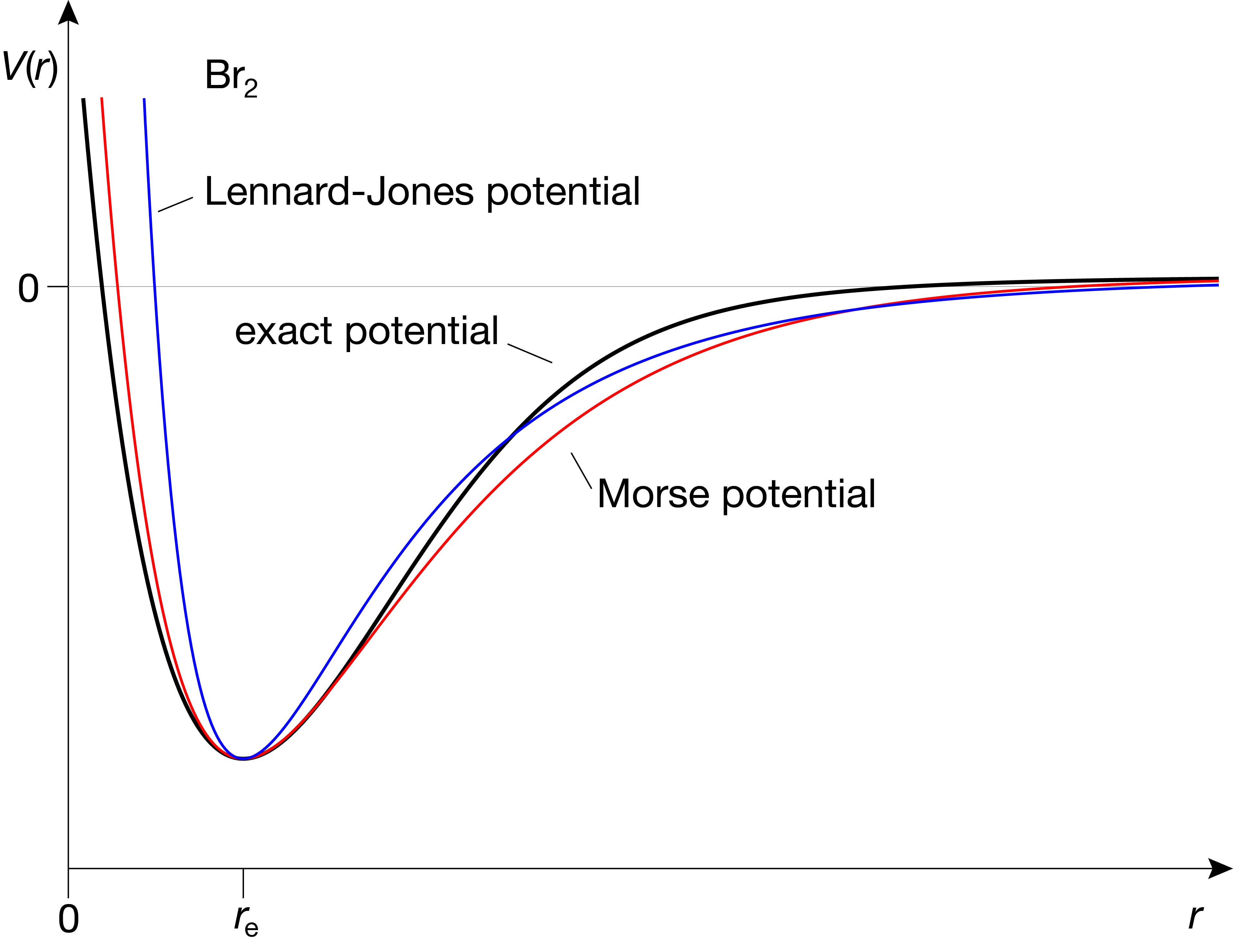
Figure 4.10 Approximating the potential of a diatomic molecule, Br₂, using the Morse potential and the Lennard-Jones potential.

4.7. Normal modes

For molecules larger than diatomics, the degree of structural flexibility grows rapidly with the number of atoms, \(N\). Each atom can move in three independent directions, therefore the total number of degrees of freedoms is \(3N\). Three of these are translations, movements of the entire molecule in one of the three orthogonal directions. Next, there are rotational degrees of freedom. A linear molecule (such as HF or CO or HCN) can rotate around two separate axes that are perpendicular to the bond, and a nonlinear molecule (such as H₂O) can rotate around 3 perpendicular axes. This is illustrated in Figure 4.11.

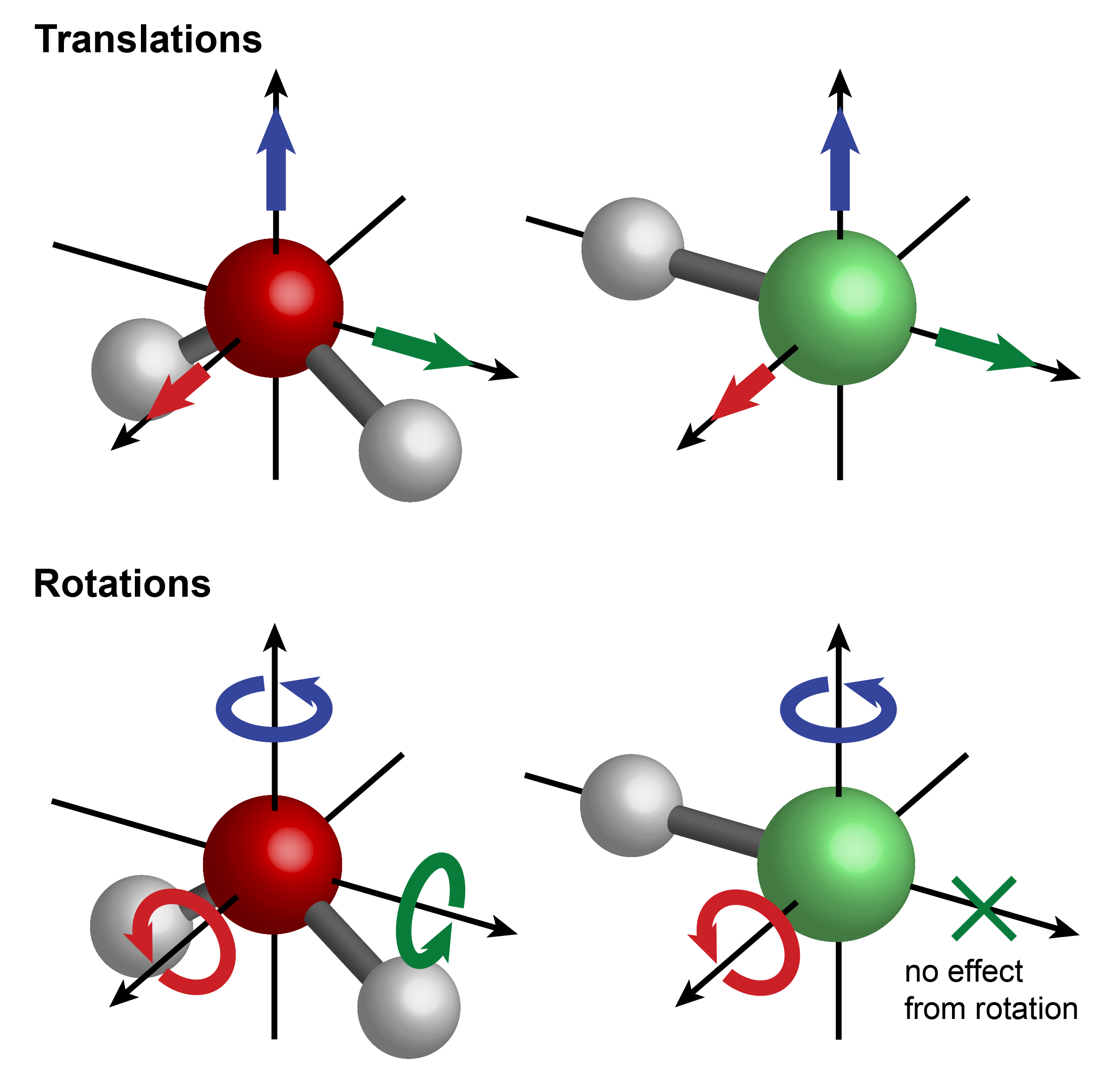
Figure 4.11 Translational and rotational degrees of freedom of water (left) and HCl (right).

The remaining degrees of freedom constitute internal degrees of freedom or vibrational degrees of freedom. Their number is given by

(4.20)\[\begin{split}\text{internal d.o.f.} = \begin{cases} 3N - 6\quad (\text{nonlinear molecule})\\ 3N - 5\quad (\text{linear molecule}) \end{cases}\end{split}\]

Since the molecular geometry can distort along each of these degrees of freedoms, these constitute vibrational normal modes. They are independent vibrations that can simultaneously occur in a molecule

For each normal mode, there is a vibrational quantum number. The vibrational state is characterized by the set of all these quantum numbers \(n_i\), and the energy is the sum over all normal-mode energies:

(4.21)\[E_{n_1,n_2,\dots} = \hbar\omega_{\mathrm{e},1}(n_1+1/2) + \hbar\omega_{\mathrm{e},2}(n_2+1/2) + \cdots\]

In the vibrational ground state, all quantum numbers are zero. The associated ground state energy, the zero-point energy is the sum over all \(\hbar\omega_{\mathrm{e},i}/2\). For a large molecule, this vibrational zero-point energy can be substantial.

As an example, consider water, H₂O, a non-linear molecule. The number of atoms is \(N=3\), and the number of normal modes is \(3\cdot3-6 = 3\). They are illustrated in Figure 4.12. Two of the modes involve only stretching (and compressing) of bond lengths, and the third mode involves bending of the bond angle.

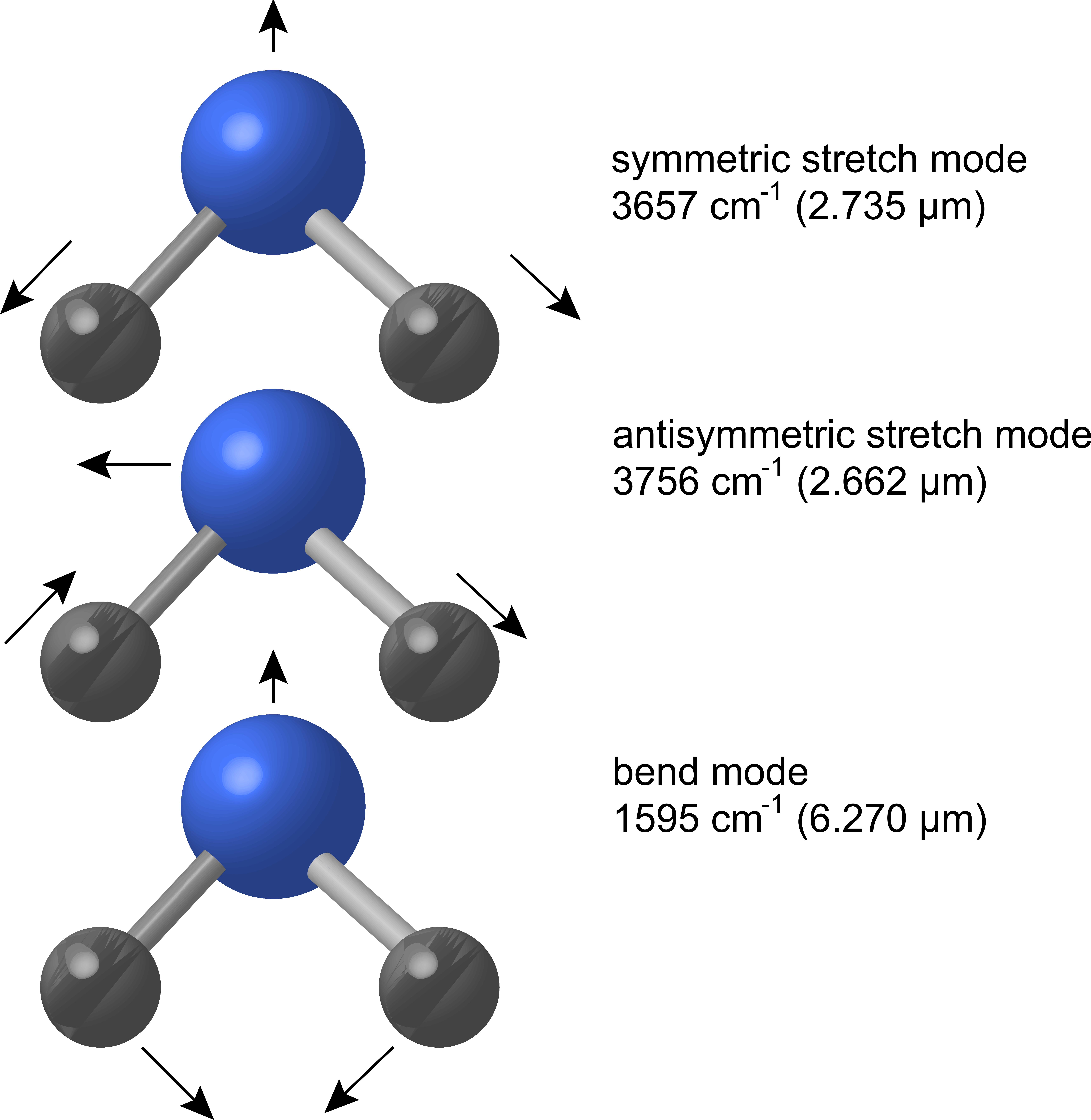
Figure 4.12 The three vibrational normal modes of water, with the corresponding wavenumbers and wavelengths.

Note

Let us calculate the vibrational energy of a water molecule in the excited vibrational state \((1,3,2)\), i.e. \(n_\mathrm{ss}=1\), \(n_\mathrm{as}=3\), and \(n_\mathrm{b}=2\). It is the sum over the energies in each of the 3 normal modes:

(4.22)\[E_{1,3,2} = \hbar\omega_{\mathrm{e,ss}}(1+1/2) + \hbar\omega_{\mathrm{e,as}}(3+1/2) + \hbar\omega_{\mathrm{e,b}}(2+1/2)\]

or, using wavenumbers,

(4.23)\[E_{1,3,2} = hc\tilde\nu_{\mathrm{e,ss}}(1+1/2) + hc\tilde\nu_{\mathrm{e,as}}(3+1/2) + hc\tilde\nu_{\mathrm{e,b}}(2+1/2)\]

For small molecules such as water, it is possible to reason about the nature of the normal modes, but for larger ones, numerical calculations are necessary to determine them. Often, the modes are spread over the entire molecule, i.e. the “displacement” for a mode involves movements of many atoms, with varying relative amplitude. The nature of a mode is commonly designaed based on the visual appearance of this movement. Besides “stretch” and “bend”, other names for vibrational motions are “wag”, “rock”, “bend”, “twist”, “pucker”, “breath”.