8. Atoms

In the previous chapter, we considered atoms with a single electron (H, He⁺). The Hamiltonian for such atoms contains one kinetic-energy term and one potential-energy term. There are four internal degrees of freedom ($r$, $\theta$, $\varphi$, and spin), and we were able to solve the time-independent Schrödinger equation analytically.

In this chapter, we move on to consider atoms with more than one electron. For these, we need an additional type of term into the Hamiltonian, the electrostatic repulsion energy between electrons.

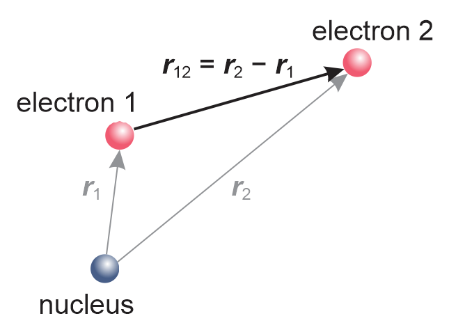
Figure 8.1 Two electrons around a nucleus form a two-electron atom. The vectors ${\mathit{r}}_1$, ${\mathit{r}}_2$ and ${\mathit{r}}_{12}$ define the relative positons of the three particles.

Take a pair of electrons, as shown in Figure 8.1. The electrostatis repulsion energy between the two is

(8.1)$$V({\mathit{r}}_1,{\mathit{r}}_2)=+\frac{1}{4\pi {ϵ}_0}\frac{e^2}{|{\mathit{r}}_1-{\mathit{r}}_2|}=+\frac{1}{4\pi {ϵ}_0}\frac{e^2}{r_{12}}$$

where ${\mathit{r}}_1$ and ${\mathit{r}}_2$ are the positions of the two electrons, and $r_{12}$ indicates the distance between the two electrons. This potential energy is always positive - it raises the overall energy. It is inversely proportional to the distance between the electrons - the closer the electrons, the higher the repulsion energy.

Note

For a sense of scale: The electrostatic repulsion energy of two electrons that are 1 Å apart is +14.4 eV.

8.1. Hamiltonian and wavefunctions

Let us now set up the Hamiltonian for a two-electron atom (such as He or Li⁺). We need to include one kinetic and one electron-nuclear attraction potential energy term for each electron, and we also need one electron-electron repulsion term:

(8.2)$$\hat{H}=-\frac{{\hslash }^2}{2m_{\mathrm{e}}}{\mathrm{\nabla }}_{\mathrm{e}1}^2-\frac{{\hslash }^2}{2m_{\mathrm{e}}}{\mathrm{\nabla }}_{\mathrm{e}2}^2-\frac{Z{e}^2}{4\pi {ϵ}_0{r}_1}-\frac{Z{e}^2}{4\pi {ϵ}_0{r}_2}+\frac{e^2}{4\pi {ϵ}_0{r}_{12}}$$

Each of the electrons has 4 degrees of freedom, making a total of 8. Therefore, the wavefunction describing the whereabouts of the two electrons depends on 8 variables.

(8.3)$$\Psi (x_1,y_1,z_1,m_1,x_2,y_2,z_2,m_2)\text{or}\Psi (r_1,{\theta }_1,{\varphi }_1,m_1,r_2,{\theta }_2,{\varphi }_2,m_2)$$

(depending whether we choose Cartesian or spherical coordinates). $\Psi$ (upper-case psi) is used to indicate a multi-electron wavefunction, to distinguish it from a one-electron wavefunction (orbital) $\psi$ (lower-case psi). This wavefunction is not defined in ordinary 3D space anymore - it is defined over an 8-dimensional space that is called configuration space. For this two-electron wavefunction, the probability interpretation is as follows. $|\Psi (x_1,y_1,z_1,m_1,x_2,y_2,z_2,m_2){|}^2$ is the probability density, and

(8.4)$$|\Psi (x_1,y_1,z_1,m_1,x_2,y_2,z_2,m_2){|}^2\mathrm{d}{x}_1\mathrm{d}{y}_1\mathrm{d}{z}_1\mathrm{d}{x}_2\mathrm{d}{y}_2\mathrm{d}{z}_2$$

represents the probability of finding electron 1 with spin projection $m_1$ in an infinitesimal volume around $(x_1,y_1,z_1)$ and electron 2 with spin projection $m_2$ in an infinitesimal volume around $(x_2,y_2,z_2)$.

To simplify notation, we introduce the following shorthand for the above wavefunction:

(8.5)$$\Psi (1,2)$$

where 1 is an abbreviation for all coordinates of electron 1 ($x_1$, $y_1$, $z_1$, $m_1$), and 2 for all coordinates for electron 2 ($x_2$, $y_2$, $z_2$, $m_2$).

In an atom with $N$ electrons, the wavefunction $\Psi$ is a function of $4N$ coordinates. The Hamiltonian for such a system has $N$ kinetic-energy terms, $N$ attraction terms, and $N(N-1)/2$ repulsion terms, one for each pair of electrons. With such a Hamiltonian, the time-independent Schrödinger equation cannot be solved analytically for $\Psi$.

Note

Consider the neutral Ne (neon) atom. It has 10 electrons, $N=10$. The Hamiltonian has 10 kinetic-energy terms, 10 attraction terms, and 45 repulsion terms. The associated 10-electron wavefunction $\Psi (1,2,3,...,10)$ depends on 40 coordinates (30 spatial, and 10 spin). The Hamiltonian and the wavefunction are monstruous already for a single atom with not a lot of electrons!

8.2. Orbital approximation

In a multi-electron atom or molecule, the potential energy for one electron depends on the exact positions of all other electrons. Since electrons repel each other, they tend to avoid each other, and the positions of the electrons depend on each other: for example, if one electron is on the left, the other one tends to be on the right. This effect is called electron correlation, and it makes it impossible to solve the Schrödinger equation analytically.

To still obtain some insight, the following approximation is made: It is assumed that each electron moves in the average electrostatic field due to all the other electrons. This is called the mean-field approximation or orbital approximation.

Note

The orbital approximation is at the heart of chemical thinking and reasoning. It connects quantum theory with chemistry.

Figure 8.2 illustrates this for a two-electron atom. Within the orbital approximation, for the purpose of determining the whereabouts of electron 2, electron 1 is assumed delocalized. Repulsion is calculated not between electron 2 and electron 1, but between electron 2 and the static continuous charge distribution corresponding to the probability density of electron 1. In essence, the electrons are treated as if their positions were uncorrelated. Of course, this is a severe approximation, since this completely neglects electron correlation. In practice, the approximation is surprisingly useful.

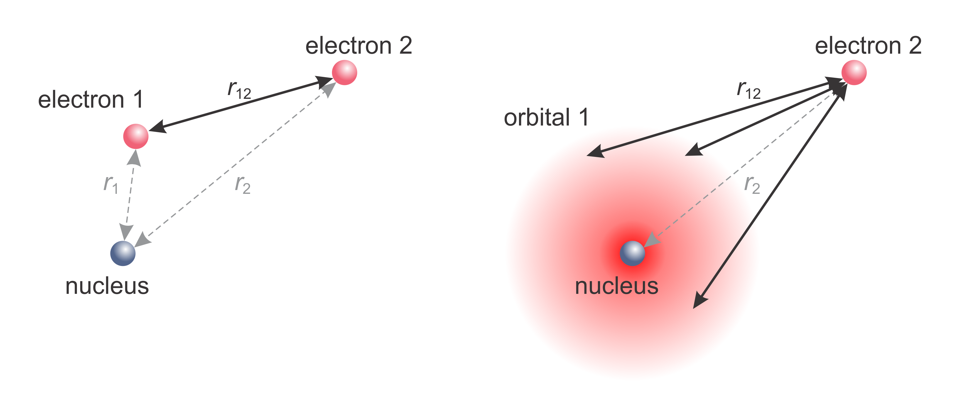
Figure 8.2 The orbital approximation. Left: The instantaneous location of two electrons. Right: In the orbital approximation, electron 1 is modeled as a continuous charge distribution delocalized based on its orbital, and the repulsion energy of electron 2 from electron 1 is calculated as the average repulsion over the charge distribution of electron 1.

The main mathematical benefit of the orbital approximation is that the many-electron wavefunction can be written in terms of products of one-electron wavefunctions (orbitals), such as

(8.6)$${\psi }_a(1)\cdot {\psi }_b(2)$$

Here, chemists say that “electron 1 is in orbital ${\psi }_a$”, and “electron 2 is in orbital ${\psi }_b$”. The list of orbitals that included in this wavefunction is called the electron configuration.

Note

For example, $(1\mathrm{s}\alpha {)}^1(1\mathrm{s}\beta {)}^1$, or shorter ${1\mathrm{s}}^2$, indicates that there is one electron in the $1\mathrm{s}\alpha$ spinorbital and one electron in the $1\mathrm{s}\beta$ spinorbital. In quantum theoretical words, this means that the overall wavefunction includes the orbitals ${\psi }_{1\mathrm{s}\alpha }$ and ${\psi }_{1\mathrm{s}\beta }$, and no others.

The effective repulsion potential energy function due to electron 1 acting on electron 2 is spherically symmetric, so that the spatial wavefunction for electron 2 can be approximated by

(8.7)$${\psi }_a(r_2,{\theta }_2,{\varphi }_2)=\frac{1}{\sqrt{\pi }}{\left(\frac{\zeta }{a_0}\right)}^{3/2}{\mathrm{e}}^{-\zeta r_2/a_0}$$

$\zeta$ (Greek letter lower-case zeta) is the effective nuclear charge. This is smaller than the actual nuclear charge $Z$, since electron 1 shields electron 2 from the nuclear charge.

For atoms and molecules with more than 2 electrons, the reasoning is not quite as simple anymore.

8.3. Pauli principle and Slater determinants

The above product form of the 2-electron wavefunction is not quite physically correct. Electrons are indistinguishable, since all their intrinsic properties are identical (same charge, mass, spin, size). Therefore, labeling one electron as 1 and the other as 2 should give the same results as labeling the first one as 2 and the other one as 1. In other words, when two electron coordinates are exchanged in the wavefunction $\Psi (1,2)$, there should be no observable changes. In particular, the probability density must remain unaffected:

(8.8)$$|\Psi (1,2){|}^2=|\Psi (2,1){|}^2$$

The Hamiltonian is of course unaffected ($\hat{H}(1,2)=\hat{H}(2,1)$), since swapping coordinates just changes the order of the terms.

Note

When two electron coordinates are exchanged (swapped), the wavefunction $\Psi (1,2)$ changes in one of three different ways. The three cases are

• $\Psi (2,1)=+\Psi (1,2)$ - The wavefunction is unchanged. It is called symmetric with respect to exchange.

• $\Psi (2,1)=-\Psi (1,2)$ - The wavefunction changes sign. It is called antisymmetric with respect to exchange.

• $\Psi (2,1)\ne \pm \Psi (1,2)$ - The wavefunction changes completely. It is neither symmetric nor antisymmetric with respect to exchange.

It turns out that, in order to be consistent with experimental observations, a many-electron wavefunction must change sign (= be antisymmetric) with respect to the exchange of the coordinates of any two electrons. This is the Pauli principle, or antisymmetrization postulate. For two electrons, it requires

(8.9)$$\Psi (2,1)=-\Psi (1,2)$$

For a valid three-electron wavefunction, the Pauli principles requires $\Psi (2,1,3)=-\Psi (1,2,3)$, $\Psi (3,2,1)=-\Psi (1,2,3)$, and $\Psi (1,3,2)=-\Psi (1,2,3)$.

More generally, a multi-particle wavefunction must be antisymmetric under the exchange of two identical fermions (electrons, protons, neutrons), and it must be symmetric under the exchange of two bosons (photons, ⁴He nuclei, etc.). Interestingly, all fermions have half-integer spin, and all bosons have integer spin.

Note

Let’s check whether the wavefunction for the electron configuration (1s$\alpha$)² satisfies the Pauli principle. The wavefunction is

(8.10)$$\Psi (1,2)={\psi }_{1\mathrm{s}}(1)\alpha (1)\cdot {\psi }_{1\mathrm{s}}(2)\alpha (2)$$

Exchanging the electron coordinates 1 and 2 gives the new wavefunction

(8.11)$$\Psi (2,1)={\psi }_{1\mathrm{s}}(2)\alpha (2)\cdot {\psi }_{1\mathrm{s}}(1)\alpha (1)$$

This is identical to the starting wavefunction! This $\Psi$ is symmetric under the exchange of two electron coordinates. It doesn’t satisfy the Pauli principle. Therefore, it does not represent a physically possible state.

This example illustrates another general principle that derives from the antisymmetrization postulate: The Pauli exclusion principle states that no two electrons can be in the same spinorbital - the orbitals must differ in at least one quantum number. This principle is the application of the more general Pauli principle to wavefunctions within the orbital approximation.

Let us examine the electron configuration (1s)² = (1s$\alpha$)(1s$\beta$). The two possible product wavefunctions are 1s$\alpha$(1)1s$\beta$(2) and 1s$\alpha$(2)1s$\beta$(1). (For notational convenience, we write ${\psi }_{1\mathrm{s}}(1)$ as 1s(1), etc.) However, they are neither symmetric nor antisymmetric under the exchange of the two electron coordinates, and therefore not physical. However, we can take the difference of the two, giving

(8.12)$$1\mathrm{s}(1)\alpha (1)1\mathrm{s}(2)\beta (2)-1\mathrm{s}(2)\alpha (2)1\mathrm{s}(1)\beta (1)$$

This wavefunction is antisymmetric under coordinate exchange and therefore represents a physical state. The sum of the two product functions gives a wavefunction that is symmetric under exchange, which is nonphysical.

A general recipe for constructing an antisymmetric multi-electron wavefunction with $N$ electrons from orbitals is the Slater determinant:

(8.13)$$\begin{array}{r}\Psi (1,2,\dots ,N)=\frac{1}{\sqrt{N!}}\left|\begin{array}{ccc}{\psi }_1(1)& \dots & {\psi }_N(1)\\ ⋮& \ddots & ⋮\\ {\psi }_1(N)& \dots & {\psi }_N(N)\end{array}\right|\end{array}$$

(See the Appendix for details on determinants.) When expanded, this determinant gives a linear combination of $N!$ products of one-electron wavefunctions (spinorbitals), with linear-combination coefficients of $+1$ and $-1$. The prefactor is the normalization factor.

Note

The Slater determinant for the two-electron configuration (1s$\alpha$)(1s$\beta$) is

(8.14)$$\begin{array}{r}\frac{1}{\sqrt{2}}\left|\begin{array}{cc}1\mathrm{s}(1)\alpha (1)& 1\mathrm{s}(1)\beta (1)\\ 1\mathrm{s}(2)\alpha (2)& 1\mathrm{s}(2)\beta (2)\end{array}\right|=\frac{1}{\sqrt{2}}[1\mathrm{s}(1)\alpha (1)1\mathrm{s}(2)\beta (2)-1\mathrm{s}(2)\alpha (2)1\mathrm{s}(1)\beta (1)]\end{array}$$

which is exactly what we arrived at before, times the normalization constant $1/\sqrt{2}$.

The Slater determinant wavefunction for 3 electrons in 3 orbitals is a linear combination of 3! = 6 products of the type ${\psi }_a{\psi }_b{\psi }_c$, and the normalization constant is $1/\sqrt{6}$.

In chemistry, we often talk about “the electron in this orbital”. Although convenient, this is inaccurate language. Looking at the Slater determinant wavefunction, there is a term for every electron in every orbital! So we cannot assign specific electrons to specific orbitals - that is exactly the Pauli principle.

8.4. Variational theorem and method

With the orbital approximation, we have introduced an approximate, but more convenient, form for the multi-electron wavefunction $\Psi$. Since it is an approximation, we will not be able to solve the time-independent Schrödinger equation exactly. Instead, we need to look for a solution that comes as close to the true wavefunction as possible within this approximation. Since the type of linear combination is fixed by the form of the Slater determinants, the unknown parts of $\Psi$ are the shapes of the orbitals.

As a starting point, we take the expectation value of energy for an arbitrary unnormalized wavefunction $\Psi$

(8.15)$$E[\Psi ]=⟨E⟩=\frac{⟨\Psi |\hat{H}|\Psi ⟩}{⟨\Psi |\Psi ⟩}$$

(The denominator is just the normalization integral.) According to the variational theorem, $E$ for any trial wavefunction $\Psi$ is always larger or at best equal to the true ground-state energy, $E_0$:

(8.16)$$E[\Psi ]\ge E_0\text{for any }\Psi$$

In addition, only for $\Psi ={\Psi }_0$ we have $E[\Psi ]=E[{\Psi }_0]=E_0$. In other words, the trial function can never be “too good”, and if it gives an energy that matches the ground-state energy, it is the ground-state wavefunction. For a proof of this theorem, see the Appendix.

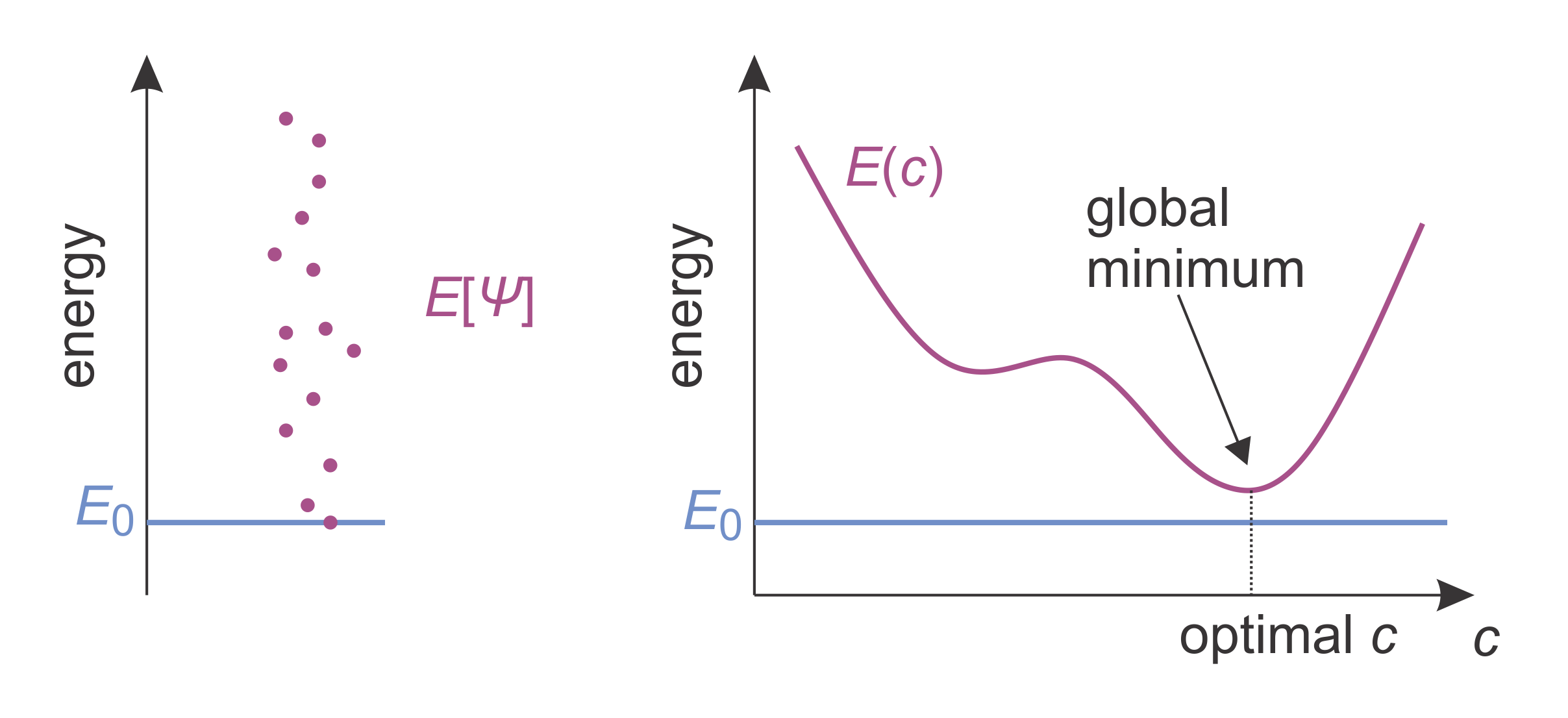
Figure 8.3 Illustrations of the variational theorem (left) and the variational method (right). The blue line indicates the true ground-state energy. The purple dots on the left indicate the energy expectation values for different trial wavefunctions. The purple curve on the right indicates the energy expectation value of a trial wavefunction that depends on a parameter $c$. There is a value $c$ where the energy expectation value is minimal (though still larger than the ground-state energy).

The variational method utilizes this theorem: Set up a trial wavefunction with adjustable parameters, e.g. $\Psi (1,2,...,c_1,c_2,...)$, where $c_1$, $c_2$, etc. are the variational parameters. Then, determine the parameter values that minimize the energy. That is, solve

(8.17)$$\frac{\partial E}{\partial c_i}=0$$

for $c_i$. The associated energy and wavefunction are the best possible approximations to $E_0$ and ${\Psi }_0$, given the choice of adjustability.

Note

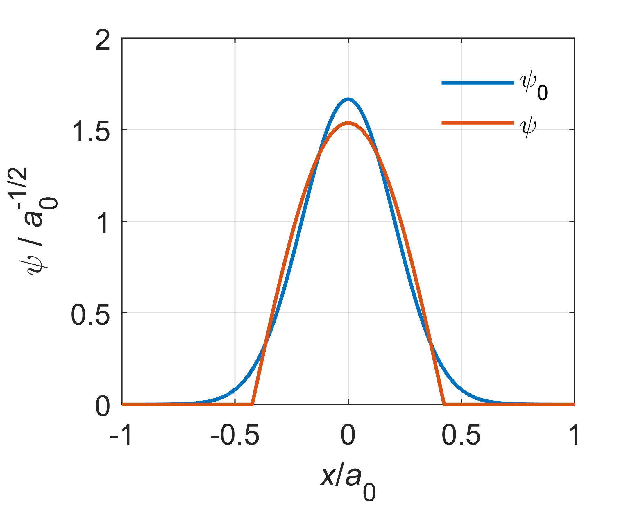
Here is an example of the variational method, applied to the harmonic oscillator. Of course, for this the variational method is not needed as we know the exact ground-state energy and wavefunction. However, the example illustrates how the variational method works. Let’s take the trial function

(8.18)$$\begin{array}{r}\psi (x)=\{\begin{array}{ll}N\cos (cx)& \text{for }|x|\le \pi /2c\\ 0& \text{otherwise}\end{array}\end{array}$$

where $N$ is the normalization constant and $c$ is the variational parameter. We can determine its optimum value using the variational method. First, we calculate the energy expectation value:

(8.19)$$E[\psi ]=\frac{{\int }_{-\mathrm{\infty }}^{\mathrm{\infty }}{\psi }^{\ast }\hat{H}\psi \mathrm{d}x}{{\int }_{-\mathrm{\infty }}^{\mathrm{\infty }}{\psi }^{\ast }\psi \mathrm{d}x}=\cdots =\frac{{\hslash }^2}{2\mu }{c}^2+(\frac{{\pi }^2}{24}-\frac{1}{4})\frac{k}{c^2}=E(c)$$

Solving $\mathrm{d}E(c)/\mathrm{d}c=0$ gives an optimal value for $c$, and the associated energy is $E(c_{\mathrm{opt}})=\cdots \approx 1.136\cdot (\hslash {\omega }_{\mathrm{e}}/2)$, which is a little higher than the exact ground-state energy $\hslash {\omega }_{\mathrm{e}}/2$. The next figure shows a plot of the associated variationally optimized wavefunction in comparison to the exact ground-state wavefunction. The approximation is pretty good.

8.5. Hartree-Fock and DFT

The Hartree-Fock method applies the variational method to an $N$-electron system with a Slater determinant wavefunction. It is applicable to both atoms and molecules. The multi-electron problem reduces to a series of coupled one-electron equations, one for each orbital:

(8.20)$$(-\frac{{\hslash }^2}{2m_{\mathrm{e}}}{\mathrm{\nabla }}^2-\frac{Z{e}^2}{4\pi {ϵ}_0}\frac{1}{r}+V_{\mathrm{eff},i}(\mathit{r})){\psi }_i(\mathit{r})={ϵ}_i{\psi }_i(\mathit{r})$$

These are called the Hartree-Fock equations, and the operator in (…) is called the Fock operator. $V_{\mathrm{eff},i}$ is the effective repulsion potential energy due to the electrons in all occupied orbitals except orbital $i$. ${ϵ}_i$ is the energy of orbital $i$.

In order to have orbitals with variable shapes, a basis set expansion is used. Each orbital is represented as an adjustable linear combination of fixed basis functions.

(8.21)$${\psi }_i(\mathit{r})=\sum _{k=1}^M{\chi }_k(\mathit{r})\cdot c_{ki}$$

Here ${\chi }_k$ are the fixed basis functions, and $c_{ki}$ are the linear combination coefficients. The shape of ${\psi }_i$ can be changed by varying the values of $c_{ki}$.

The basis functions are chosen to satisfy two criteria: (1) They should be similar in shape to the actual orbitals, so that the expansion can be short (i.e. $M$ is small), and (2) they should be mathematically easy to deal with, in particular it should be easy to evaluate integrals involving these functions. The functions that match these criteria best are linear combinations (contractions) of Gaussian functions. These are called Gaussian-type orbitals (GTOs). For a s orbital:

(8.22)$$\chi (\mathit{r})=N\sum _q{d}_q{\mathrm{e}}^{-{\alpha }_q{r}^2}$$

The ${\alpha }_q$ are the exponents, and $d_q$ are called contraction coefficients. Figure 8.4 illustrates a 1s function for a hydrogen atom, composed as a linear combination of three Gaussians.

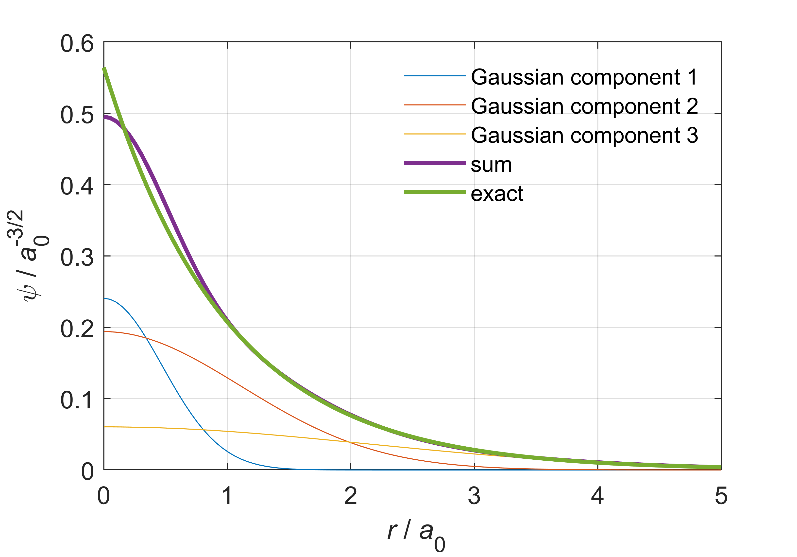
Figure 8.4 A Gaussian basis function representing the 1s orbital of a hydrogen atom. The function is a linear combination of three Gaussians. The exact wavefunction is shown as well.

In the variational method for determining the optimal wavefunction and energy for the ground state, the basis functions ${\chi }_k$ are kept fixed, and the MO coefficients $c_{ki}$ are determined, subject to the constraint that the orbitals need to be orthonormal.

There is an issue with solving the Hartree-Fock equations: The potential $V_{\mathrm{eff},i}$ in the Hartree-Fock equation for orbital ${\psi }_i$ can only be calculated if all the other orbitals are known, but those in turn require the knowledge of orbital ${\psi }_i$. Therefore, the equations cannot be solved directly in a single step. Instead, an iterative procedure called the self-consistent field (SCF) method is used: At the outset, approximate forms of all orbitals are guessed, and the associated $V_{\mathrm{eff},i}$ are calculated. Then the Hartree-Fock equations are solved to give a new set of orbitals (and their associated orbital energies), from which new $V_{\mathrm{eff},i}$ are calculated. This procedure is repeated iteratively until it converges, i.e. until the orbitals ${\psi }_i$ and the total energy do not change significantly any more from iteration to iteration. Figure 8.5 shows a flowchart of the SCF method.

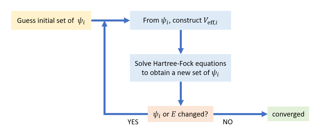
Figure 8.5 The self-consistent field (SCF) method for solving the Hartree-Fock equations to obtain atomic and molecular orbitals.

Density functional theory (DFT) is a related variational method to calculate ground-state wavefunctions and energies. Like Hartree-Fock, it uses a Slater-determinant wavefunctions with orbitals, and it uses an SCF procedure. It differs from Hartree-Fock by adding semiempirical terms (so-called exchange-correlation functionals) to the Hamiltonian. These correction terms are designed to re-capture some of the electron-electron correlation effects that are neglected due to the use of a Slater determinant as the wavefunction. There is a large number of different exchange-correlation functionals that are referred to by acronyms, such as B3LYP, PBE, M06, etc. With the augmented Hamiltonian, DFT yields generally better results than Hartree-Fock. Hartree-Fock and DFT are just two methods of a large collection of ab initio methods (ab initio = from first principles) for solving the Schrödinger equation for atoms and molecules. Among these, DFT is by far the most broadly employed method.

8.6. Multi-electron atoms

Using the methods above, it is now possible to calculate the electronic structure of all atoms of the periodic table. The wavefunction for each atom is a Slater determinant built from orbitals that resemble the hydrogen orbitals in their angular shape, although they differ in their radial extent. The orbital energies ${ϵ}_i$ depend on $n$, $l$, and on $Z$. The higher the nuclear charge, the lower the energy of a particular orbital.

Whereas all states in the hydrogen atom with equal $n$ are essentially degenerate (apart from the tiny splitting due to spin-orbit coupling), this no longer holds for the orbitals of the same name in multi-electron atoms. The electron-electron repulsion breaks this symmetry.

The sequence of occupied orbitals in an atom is given by the Aufbau principle (“Aufbau” is German for “buildup” or “construction”): To obtain the ground-state electron configuration for an atom (or molecule) with $N$ electrons, fill the $N$ lowest-energy spin-orbitals. For neutral atoms, this is summarized by the Madelung rule, which is illustrated in Figure 8.6. The sequence is: 1s, 2s, 2p, 3s, 3p, 4s, 3d, 4p, etc. This rule holds for most neutral atoms, but has exceptions: It does not work for some neutral atoms further down on the periodic table (Cu is an example). Also, it does not apply to cations or anions.

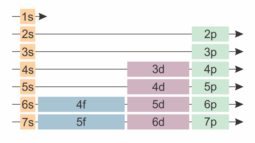
Figure 8.6 The sequence in which atomic orbitals are filled, according to the Madelung rule, indicated by the arrows starting on the top left. Note the similarity to the periodic table.

Note

A neutral carbon atom has 6 electrons. The Madelung rule predicts the ground-state electron configuration (1s)²(2s)²(2p)².

Note

The rule has many exceptions. For example, consider Mn and Co ²⁺, both of which have 25 electrons. According to the rule, both should have the same electron configuration. Indeed, the experimentally determined electron configuration for Mn is [Ar]4s²3d⁵, as predicted by the rule. However, for Co²⁺ it is [Ar]3d⁷ (not consistent with the rule). [Ar] indicates the electron configuration of argon (18 electrons): [Ar] = 1s² 2s²2p⁶3s²3p⁶.

Besides dictating the sequence of filling with electrons, orbital energies have another specific use. According to the Koopmans theorem, the energy of the highest occupied orbital is approximately equal to the ionization energy ( = energy required to extract an electron from the atom). For example, if the orbital energy is -2.3 eV, then the ionization energy is approximately 2.3 eV. On the other hand, the energy of the lowest unoccupied orbital is approximately equal to the electron affinity, i.e. the energy released when an electron is added to an atom. Knowing these two energies for any atom (or molecule) allows the prediction of the direction of electron transfer, as illustrated in Figure 8.7.

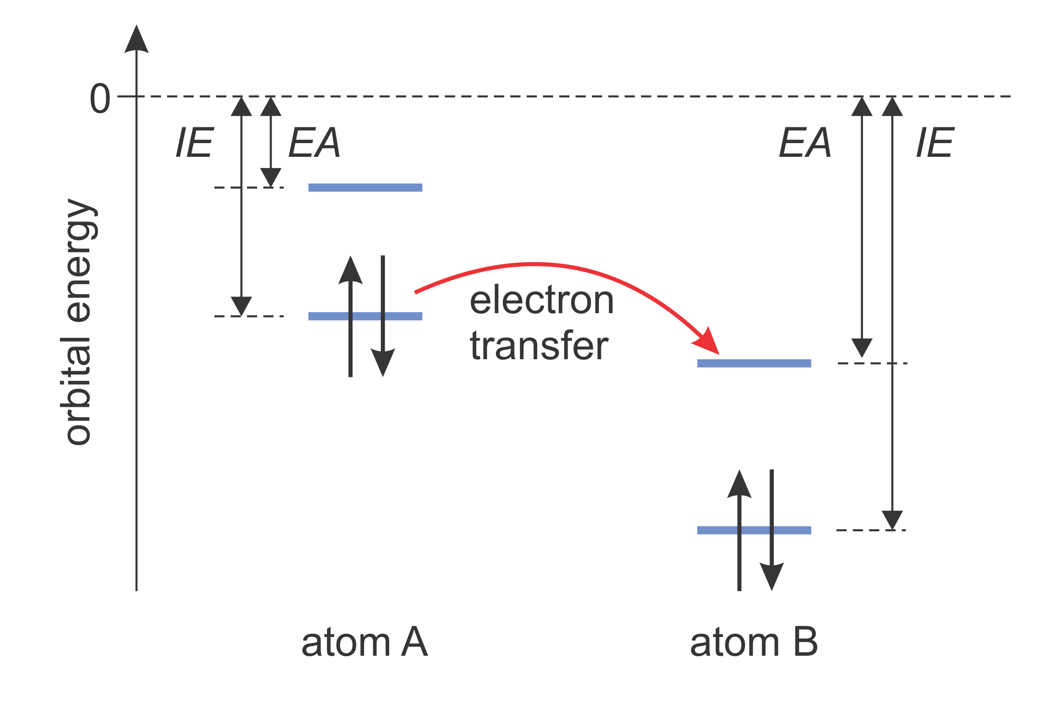
Figure 8.7 Ionization energy (IE) and electron affinity (EA). Electron transfer is energetically favorable if the highest occupied orbital energy of one atom is higher than the lowest unoccupied orbital energy of the other.

One could be tempted to assume that the sum of all the occupied orbital energies is equal to the total energy of the atom. This is not the case. Summing the orbital energies double-counts the electron-electron repulsion energy and gives a value that is higher than the actual total energy. For example, in a two-electron atom, the orbital energies of both electron 1 and electron 2 include the 1-2 repulsion, which would therefore be double-counted.