9. Molecules

A molecule is an assembly of atoms held together in a stable conformation by chemical bonds. A chemical bond, in turn, is a reasonably stable connection between atoms (this definition is by Roald Hoffmann, chemistry Nobel laureate 1981). Molecules exist because their energy is lower compared to the separated constituent atoms. In this chapter, we lay out molecular orbital (MO) theory, which allows us to predict the energy and the geometric and electronic structure of molecules. Recall that a molecular orbital (MO) is a one-electron wavefunction in a molecule.

For the purpose of quantum theoretical description, a molecule is considered a collection of nuclei and electrons. The total molecular Hamiltonian for such a collection of particles is

(9.1)\[\hat{H}_\mathrm{tot} = \sum_{i} \hat{T}_{\mathrm{e},i} + \sum_{k} \hat{T}_{\mathrm{n},k} - \sum_{i,k} \hat{V}_{\mathrm{ne},ik} + \sum_{k\neq l} \hat{V}_{\mathrm{nn},kl} + \sum_{i\neq j} \hat{V}_{\mathrm{ee},ij}\]

The first and second sum collect all kinetic-energy terms, for all electrons \(i\) and all nuclei \(k\). The third term is the nuclear-electronic attraction energy, summed over all combinations of electron and nucleus. It is negative, since it is stabilizing. The fourth term combines all repulsive terms between unique pairs of nuclei. The last term describes the total electron-electron repulsion energy, which again is a sum over all unique pairs of electrons. The repulsion energy terms are positive, they raise the overall energy.

Note

For H₂O, there are 10 electrons and 3 nuclei, so there are 13 kinetic-energy terms, 30 attraction terms, 3 nuclear repulsion terms, and 45 electron-electron repulsion terms. This gives a total of 91 terms.

With such a Hamiltonian, the Schrödinger equation is unsolvable, even when using the orbital approximation (i.e. a Slater determinant form of the wavefunction). To simplify the problem, another important approximation is made. We discuss this next.

9.1. Born-Oppenheimer approximation

The Born-Oppenheimer approximation is a notion of central importance to chemistry. The reasoning for it goes as follows. Electrons and nuclei experience similar electrostatic forces in a molecule. Now, since nuclei are much more massive than electrons (e.g. the proton mass is 1836 times that of the electron), nuclei are accelerated much less by these forces. Therefore, at very short timescales (less than 10^-16 seconds), electrons move, but nuclei essentially don’t. From the point of view of the electrons, the nuclei appear frozen; and from the point of view of the nuclei, the electrons appear not as localized particles, but as a continuous delocalized distribution of negative charge.

Note

As a useful visual analogy for this, picture a nucleus as a hiker, and the surrounding electrons as mosquitoes. The mosquitoes move much faster than the hiker (unless she runs), therefore the hiker perceives them as “delocalized”, whereas the mosquitoes see the hiker as essentially stationary.

This separation of time scales allows us to separate nuclear and electron motion. This is the Born-Oppenheimer approximation. The total wavefunction \(\varPsi_\mathrm{tot}\) is written as a product of the nuclear wavefunction \(\varPsi_\mathrm{nuc}\) (which incorporates the overall translation, rotation, and all vibrations of the molecule) and the electronic wavefunction \(\varPsi\):

(9.2)\[\varPsi(\boldsymbol{r},\boldsymbol{R}) = \varPsi_\mathrm{nuc}(\boldsymbol{R})\cdot \varPsi(\boldsymbol{r};\boldsymbol{R})\]

Here, \(\boldsymbol{r}\) indicates all electron coordiantes, and \(\boldsymbol{R}\) all nuclear coordinates. The total time-independent Schrödinger equation separates into two equations, one for the nuclei, and one for the electrons:

(9.3)\[\begin{split}\hat{H}_\mathrm{tot}\varPsi_\mathrm{tot} = E_\mathrm{tot}\varPsi_\mathrm{tot} \rightarrow \begin{cases} \hat{H}_\mathrm{nuc}(\boldsymbol{R})\varPsi_\mathrm{nuc}(\boldsymbol{R}) = E_\mathrm{nuc}\cdot\varPsi_\mathrm{nuc}(\boldsymbol{R}) & \text{nuclei} \\ \hat{H}(\boldsymbol{r};\boldsymbol{R})\varPsi(\boldsymbol{r};\boldsymbol{R}) = E(\boldsymbol{R}) \cdot\varPsi(\boldsymbol{r};\boldsymbol{R}) & \text{electrons} \end{cases}\end{split}\]

where \(\boldsymbol{R}\) after the semicolon in \(\varPsi\) is a reminder that the electronic wavefunction depends on the nuclear positions.

Now a two-step solution is possible. First, the nuclei are assumed fixed at specific positions, and the Schrödinger equation for the electrons is solved, yielding the electronic wavefunction \(\varPsi\) and the electronic energy \(E\) for that specific nuclear configuration (i.e. nuclear positions). Repeating this procedure for other nuclear configurations then maps out the electronic energy as a function of nuclear configurations, \(E(\boldsymbol{R})\). This is then used in the second step as a potential-energy term in a Hamiltonian for the nuclear wavefunctions, \(\varPsi_\mathrm{nuc}(\boldsymbol{R})\). Therefore, \(E(\boldsymbol{R})\) is called a potential-energy surface.

9.2. Dihydrogen cation

The simplest molecule is the dihydrogen cation, \(\mathrm{H}_2^+\), consisting of two nuclei and one electron. The dihydrogen cation is the only one-electron molecule, and the only molecule overall, for which the electronic time-independent Schrödinger equation can be solved analytically, giving energy and wavefunction.

The electronic Hamiltonian for \(\mathrm{H}_2^+\) contains one kinetic and three potential-energy terms:

(9.4)\[\hat{H} = -\frac{\hbar^2}{2m_\mathrm{e}} \nabla^2 + \frac{e^2}{4\pi\epsilon_0} \left( -\frac{1}{r_\mathrm{a}} -\frac{1}{r_\mathrm{b}} +\frac{1}{R_\mathrm{ab}} \right)\]

Figure 9.1 gives the meaning of the various distance variables, \(r_\mathrm{a}\), \(r_\mathrm{b}\), and \(R_\mathrm{ab}\).

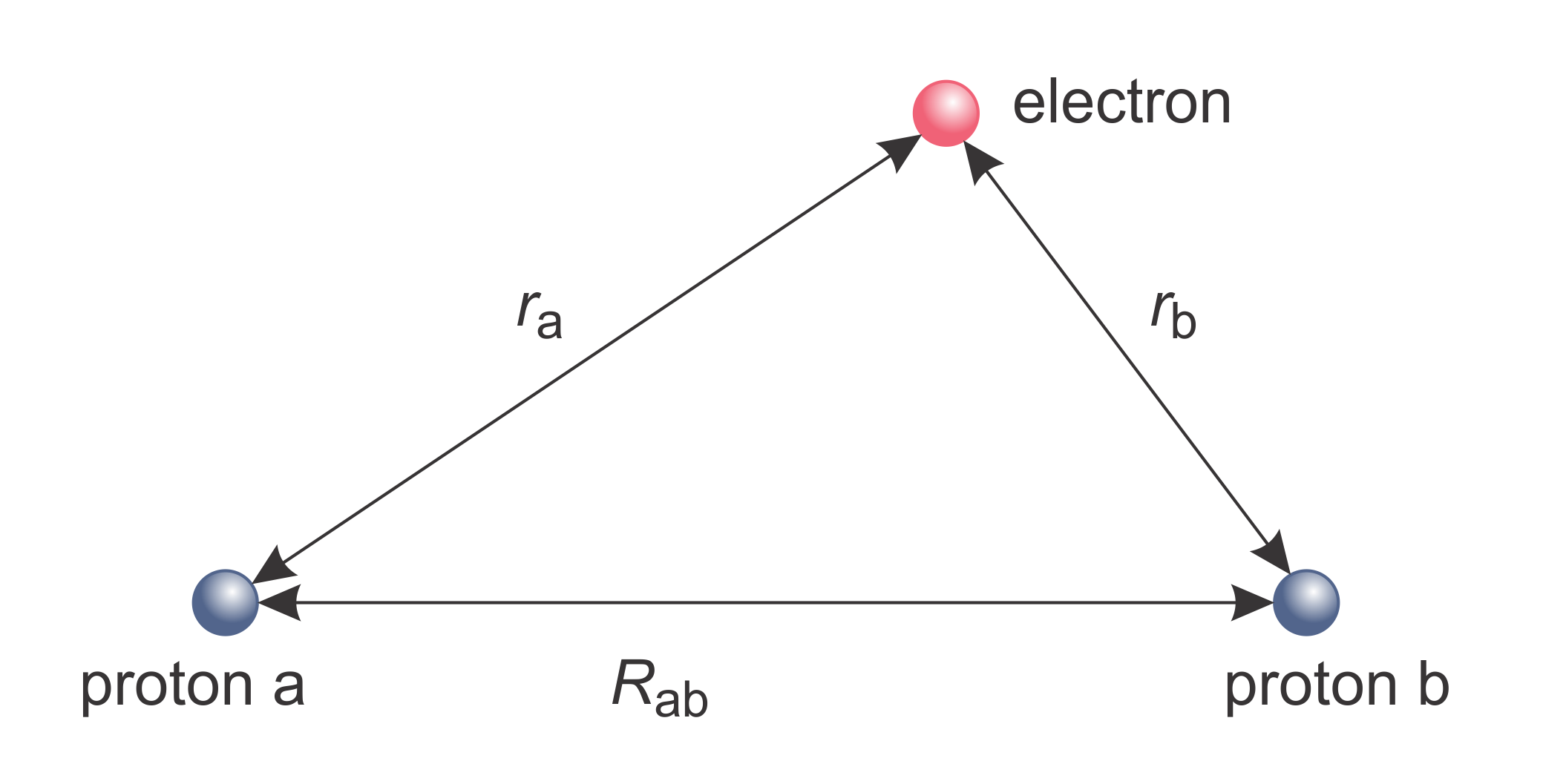
Figure 9.1 Dihydrogen cation \(\mathrm{H}_2^+\): The distances relevant for the electrostatic attraction and repulsion energies.

Energies. Solving the electronic time-independent Schrödinger equation for a range of \(R_\mathrm{ab}\) gives a set of potential energy curves \(E(R_\mathrm{ab})\), i.e. the electronic energy as a function of inter-nuclear distance. There is one curve for each state. The ones for the ground state and the first excited state are plotted in Figure 9.2.

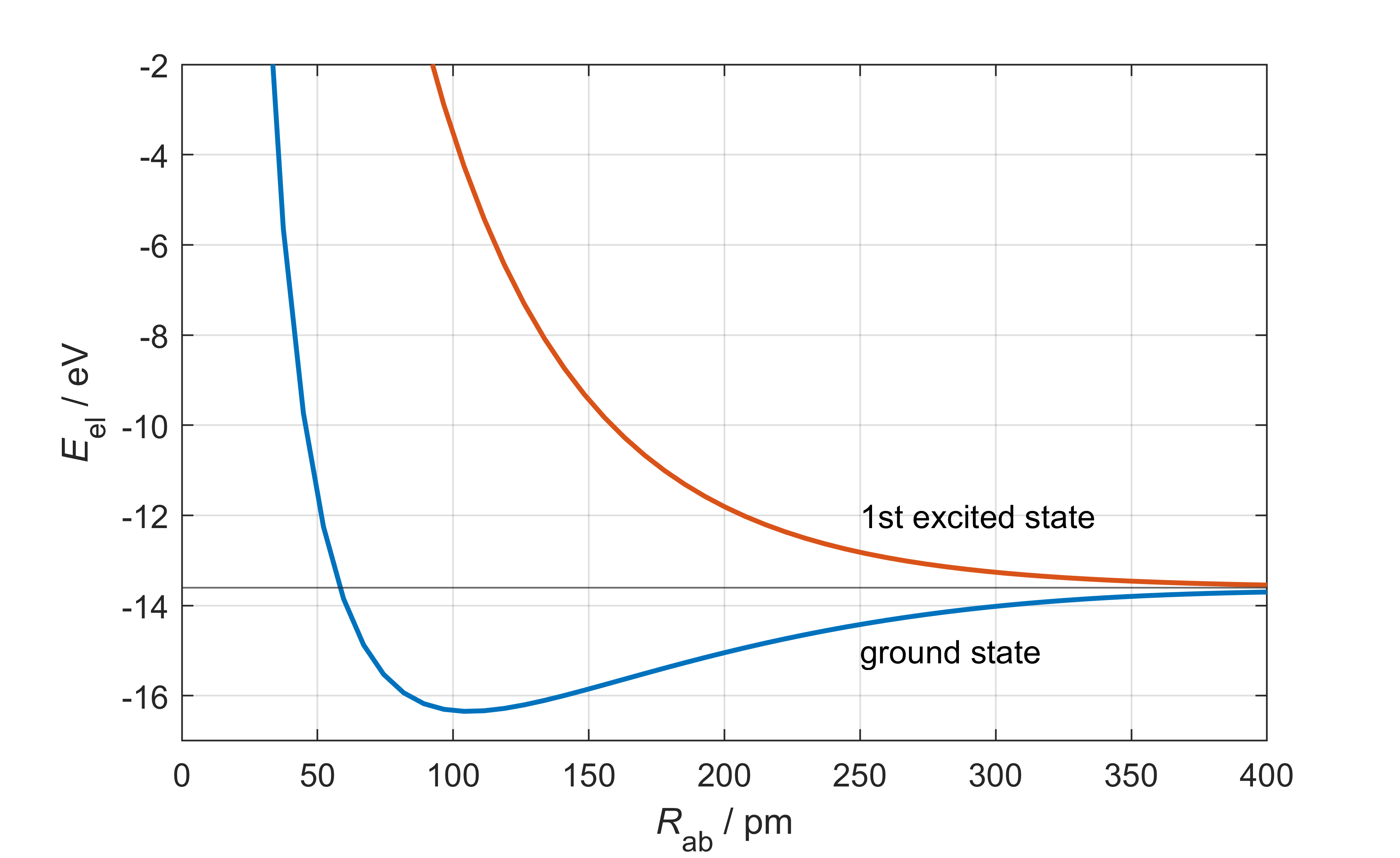
Figure 9.2 The potential-energy curves of the electronic ground state (blue) and first excited state (red) of \(\mathrm{H}_2^+\), as a function of inter-proton distance, \(R_\mathrm{ab}\). The dissociation limit -13.6 eV is also indicated.

The ground-state energy shows a minimum at about 105.7 pm, indicating that two protons and an electron form their lowest-energy state at this distance. At the minimum, the energy is -16.3 eV, about 2.7 eV lower than at infinite separation (\(R_\mathrm{ab}\rightarrow\infty\); corresponding to a hydrogen atom and a separate proton). Therefore, this molecule is stable ( = has lower energy than constitutent atoms infinitely separated). In contrast, in the first excited state the energy decreases monotonically with increasing distance, and the molecule is not stable. Such a state is called dissociative.

Wavefunctions. The wavefunction for the electronic ground state at the equilibrium geometry (105.7 pm) is shown in Figure 9.3. Near the nuclei, the wavefunction resembles closely the AOs of the constituent atoms. In addition, there is increased electron density between the two nuclei, such that the wavefunction is more delocalized than the AOs of each constituent atom.

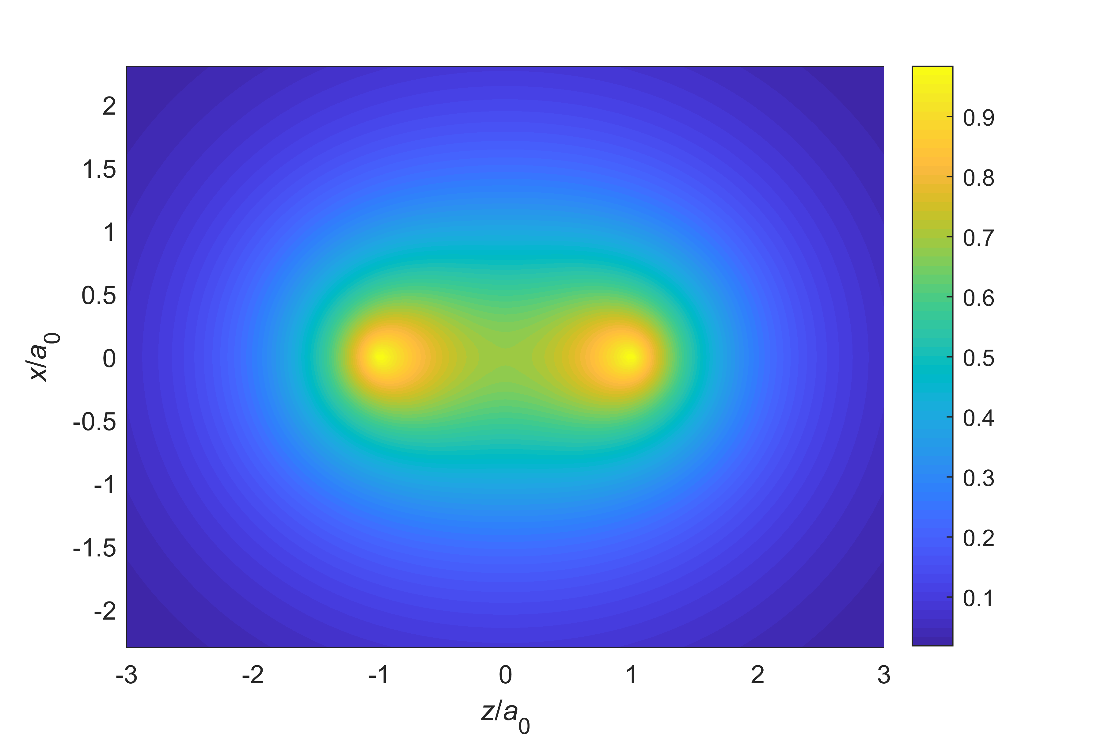
Figure 9.3 The ground-state wavefunction for the dihydrogen cation, for the equilibrium inter-nuclear distance 105.7 pm (= 2 \(a_0\)).

Note

Why is this molecule stable? There are two reasons: (a) The electron has more space to spread out in \(\mathrm{H}_2^+\) as compared to an H atom (plus distant proton). This enhanced delocalization lowers the kinetic energy (there is less curvature in the wavefunction). (b) The electron is somewhat closer to the nuclei in \(\mathrm{H}_2^+\) as compared to an H atom (plus distant proton); this lowers the potential energy. Altogether, the total energy is lowered.

A purely electrostatic explanation for the stability, in terms of increased electron density between the two nuclei, is often taught in introductury chemistry courses. It is incomplete, as is misses to take into account the electron motion. It also suggests incorrectly that the location of the lowest potential energy for the electrons is between the nuclei - that is actually close to the nuclei.

Since this is a one-electron molecule, this is a one-electron wavefunction, i.e. a molecular orbital. For molecules larger than \(\mathrm{H}^+_2\), the wavefunction is a multi-electron wavefunction, and commonly represented as a Slater determinant with molecular orbitals. Beyond \(\mathrm{H}^+_2\), molecular orbitals cannot be calculated analytically, and an additional approximation (in addition to the Born-Oppenheimer and the orbital approximation) must be introduced.

9.3. MO theory

Now, the molecular orbitals of the molecular hydrogen cation shown in Figure 9.3 look very similar to the 1s atomic orbitals near the nuclei. This suggests that a reasonable strategy for simplifying the problem and developing a general strategy for calculating MOs would be to approximate the MOs as linear combinations of AOs (LCAO). This method is called MO-LCAO and is the cornerstone of MO theory.

As a minimal example, consider the following approximate MO built from two AOs (which themselves might already be approximations - see previous chapter)

(9.5)\[\psi = c_1\phi_1 + c_2\phi_2\]

where \(\psi\) is the MO, and \(\phi_1\) and \(\phi_2\) are the AOs. The energy expectation value of this approximate MO is

(9.6)\[E = \frac{\langle\psi|\hat{H}|\psi\rangle}{\langle\psi|\psi\rangle} = \frac{c_1^2H_{11}+2c_1c_2H_{12}+c_2^2H_{22}}{c_1^2S_{11}+2c_1c_2S_{12}+c_2^2S_{22}}\]

with the abbreviations

(9.7)\[H_{ij} = \left\langle\phi_i\middle|\hat{H}\middle|\phi_j\right\rangle \qquad S_{ij} = \left\langle\phi_i\middle|\phi_j\right\rangle\]

\(H_{ij}\) are Hamiltonian matrix elements. \(H_{11}\) and \(H_{22}\) are called Coulomb integrals, and \(H_{12}\) is a resonance integral. \(S_{ij}\) are overlap integrals. If the AOs are normalized, then \(S_{11} = S_{22} = 1\), and \(S_{12}\) is between 0 and 1.

The linear-combination coefficients \(c_1\) and \(c_2\) are determined by energy minimization, based on the variational method discussed in Variational theorem and method. \(c_1\) and \(c_2\) are optimal if the energy derivatives with respect to all coefficients are simultaneously zero:

(9.8)\[\frac{\partial E}{\partial c_1}=0 \quad \text{and} \quad \frac{\partial E}{\partial c_2}=0\]

Each of these equations results in a linear equation in \(c_1\) and \(c_2\), giving a system of two linear equations. As shown in the derivation in the Appendix, this system can only be solved if the energy \(E\) satisfies the following quadratic equation

(9.9)\[E^2(S_{11}S_{22}-S_{12}^2) +E(-H_{11}S_{22}-H_{22}S_{11}+2H_{12}S_{12}) + H_{11}H_{22}-H_{12}^2 = 0\]

Solving this quadratic equation gives \(E\), and with \(E\) in hand, \(c_1\) and \(c_2\) can be calculated.

For a homodiatomic molecule (\(H_{11}=H_{22}\)) and assuming AO normalization (\(S_{11}=S_{22}=1\)), the two solutions (MOs and associated energies) are

(9.10)\[\begin{split}\begin{eqnarray} \psi_\mathrm{g} &=&\frac{1}{\sqrt{2+2S_{12}}}(\phi_1+\phi_2) & E_\mathrm{g} &=& \frac{H_{11}+H_{12}}{1+S_{12}} \\ \psi_\mathrm{u} &=&\frac{1}{\sqrt{2-2S_{12}}}(\phi_1-\phi_2)\qquad & E_\mathrm{u} &=& \frac{H_{11}-H_{12}}{1-S_{12}} \end{eqnarray}\end{split}\]

\(\psi_\mathrm{g}\) describes the ground state, and \(\psi_\mathrm{u}\) describes the first excited state.

Since the MO contains two AOs, we have two linear-combination coeffients (\(c_1\) and \(c_2\)), and we got one \(\partial E/\partial c_i\) equation for each, and therefore two linear equations, which yield two solutions. In general, N atomic orbitals yield N molecular orbitals. In order to (approximately) model higher excited states, we would need to include more than two AOs in the linear combination. The AOs in molecules serve the same purpose as the Gaussian basis functions used for atoms.

Figure 9.4 shows the accompanying orbital energy level diagram, called the MO diagram, with the case of hydrogen indicated, where \(\phi_1\) and \(\phi_2\) are 1s AOs. \(\psi_\mathrm{g}\) is called the bonding MO, since its energy is lower than the constituent AOs, and \(\psi_\mathrm{u}\) is called the antibonding MO.

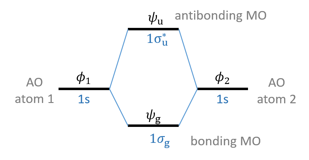
Figure 9.4 MO diagram involving two atomic orbitals.

The MOs built from two 1s atomic orbitals are shown in Figure 9.5. The sum of the two 1s AOs gives the bonding MO, with increased electron delocalization. The difference gives the antibonding MO, with reduced electron delocalization.

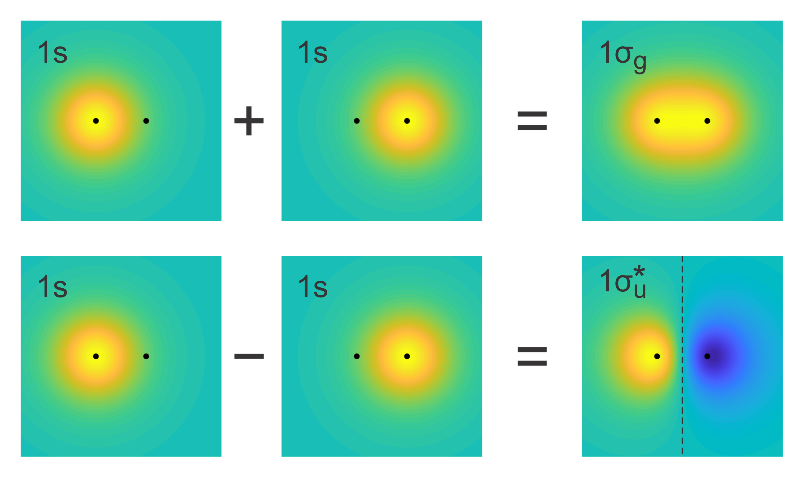
Figure 9.5 Linear combinations of two 1s atomic orbitals give a bonding MO and an antibonding MO. The black dots indicate the locations of the nuclei, and the dashed line indicates the nodal plane perpendicular to the bond. Yellow indicates positive, blue negative, and green close-to-zero values.

Figure 9.6 summarizes the nomenclature for MOs in diatomic molecules. It abbreviates information about the symmetry and the energy of the MO. The Greek letter indicates the symmetry of the MO around the bond axis: \(\sigma\) for cylindrical symmetry, \(\pi\) if the MO has one nodal plane containing the bond, and \(\delta\) if the MO features two such nodal planes. The subscript letter indicates the parity of the MO, that is, its behavior under inversion through the center of the bond: g for even (g = gerade, German for even) and u for odd (u = ungerade, German for odd). This parity only exists in homonuclear diatomic molecules, not in heternuclear diatomics. The asterisk indicates an antibonding orbital. The distinctive characteristic of any antibonding MO is the presence of a nodal plane perpendicular to the bond direction. Finally, the leading number indicates the energy order of the MO within the group of all MOs of the same symmetry.

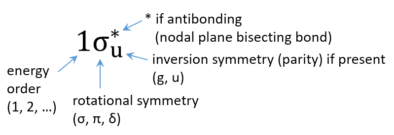
Figure 9.6 Labels for orbitals in diatomic molecules.

Note

For example, \(3\sigma_\mathrm{u}^*\) is cylindrically symmetric (\(\sigma\)), it changes sign upon inversion (parity u), it is the third \(\sigma_\mathrm{u}\) MO starting from the lowest-energy one, and it is an antibonding MO (*), i.e. it has a nodal plane that bisects the bond.

Given the MOs, the electron configuration for a given number of electrons can now be determined using the Aufbau principle (as discussed for atoms): Fill the \(N\) electrons into the \(N\) spin-orbitals of lowest energy. This is applied in Figure 9.7 to the case of different charge species of dihydrogen.

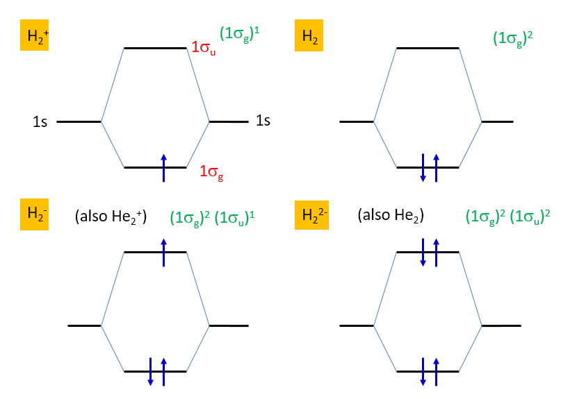
Figure 9.7 MO diagrams illustrating the Aufbau principle for the various charge species of dihydrogen. Electron configurations are shown in green.

Second-row diatomics. For second-row elements, the additional AOs from the second shell determine the bonding and antibonding MOs. The 1s AOs are more concentrated around the nuclei and do not overlap. With the 2s and 2p orbitals, several types of \(\sigma\) and \(\pi\) MOs are possible. These are shown in Figure 9.8.

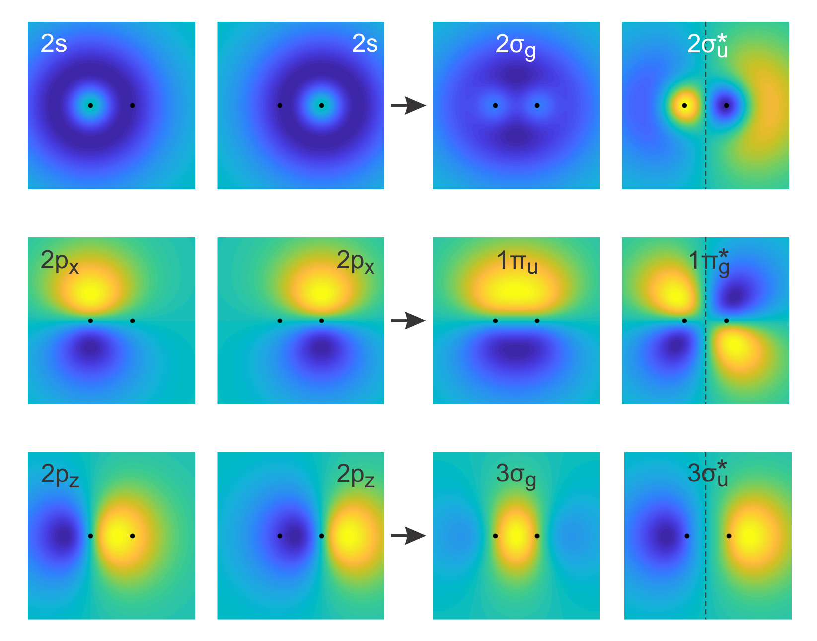
Figure 9.8 MOs contructed from linear combinations of AOs with \(n=2\). The AOs are shown on the left, and the bonding and antibonding MOs are shown on the right. The MO labels refer to homonuclear diatomic molecules (such as N₂ or O₂). The black dots indicate the locations of the nuclei, and the dashed line indicates the nodal plane perpendicular to the bond. Yellow indicates positive, blue negative, and green zero values.

The progression of MO energies in neutral homodiatomic molecules across the second row of the periodic table are shown in Figure 9.9.

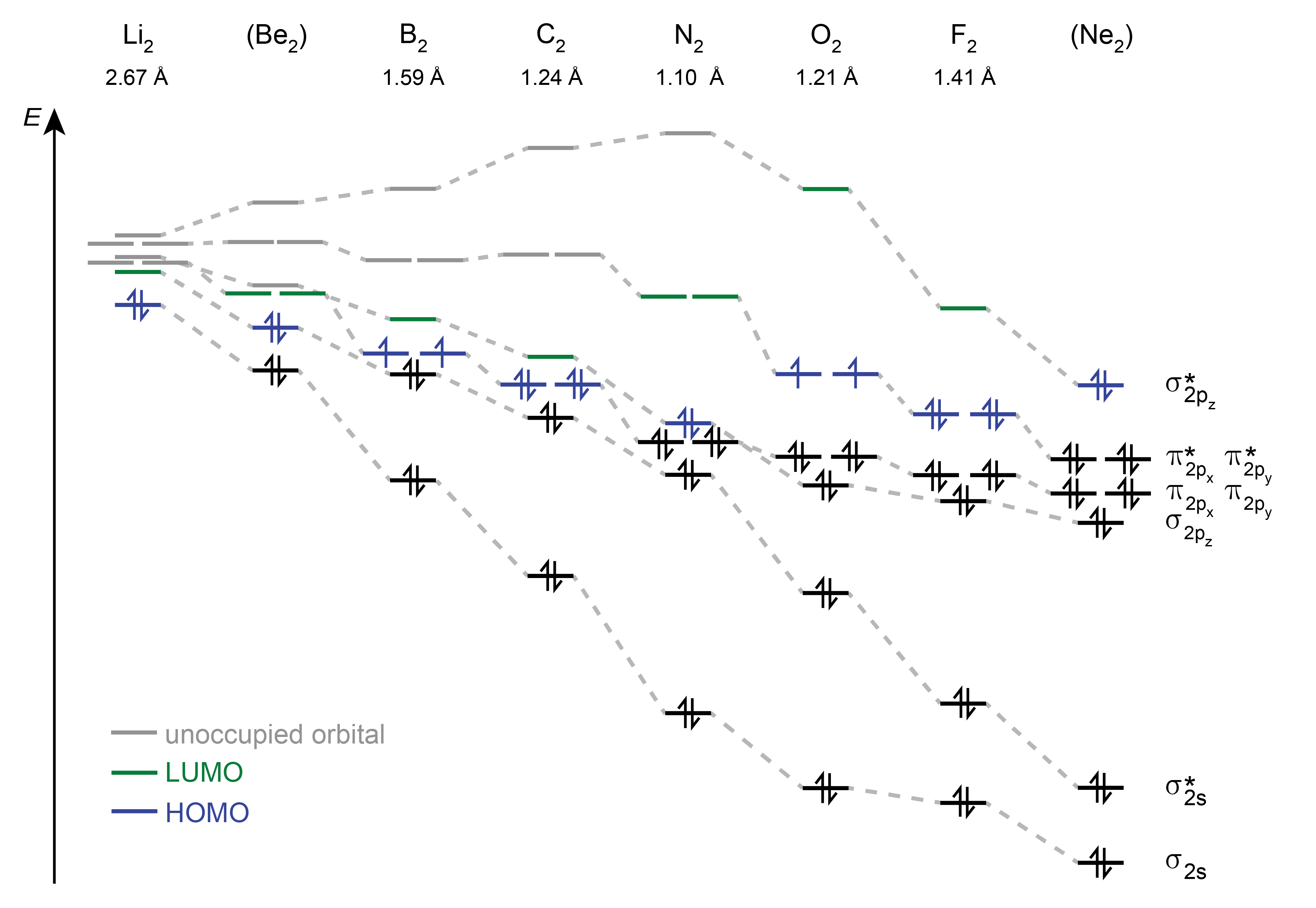
Figure 9.9 The MO diagrams of all homonuclear diatomics from Li to Ne. The two lowest-energy MOs resulting from the overlap of the 1s AOs are not shown. Note that Be₂ and Ne₂ have not been observed.

Koopmans’ theorem, as discussed in the previous chapter for atoms, applies to molecules as well. It states that the ionization energy is equal to the negative Mo energy of the HOMO. This is an approximation, as removing one electron from a molecule does not just empty the HOMO, but also leads to a slight redistribution of the remaining electrons, and therefore to shape changes in the remaining occupied orbitals. This orbital relaxation is neglected in Koopmans’ theorem. This approximation is called the frozen-core approximation.

Bond order. The bond order in a diatomic molecule is defined as

(9.11)\[\text{bond order} = (\text{# electrons in bonding MOs} - \text{# electrons in antibonding MOs})/2\]

If the total number of electrons is even, the bond order is an integer (0, 1, 2, 3). If it is odd, the bond order is a half-integer (1/2, 3/2). Figure 9.10 shows the bond orders for neutral homodiatomic molecules of the first two rows of the periodic table.

The bond order is a qualitative predictive tool. When comparing two molecules with different bond orders, the one with the higher bond order usually has (a) the higher bond dissociation energy, (b) the shorter bond length, and (c) the larger force constant.

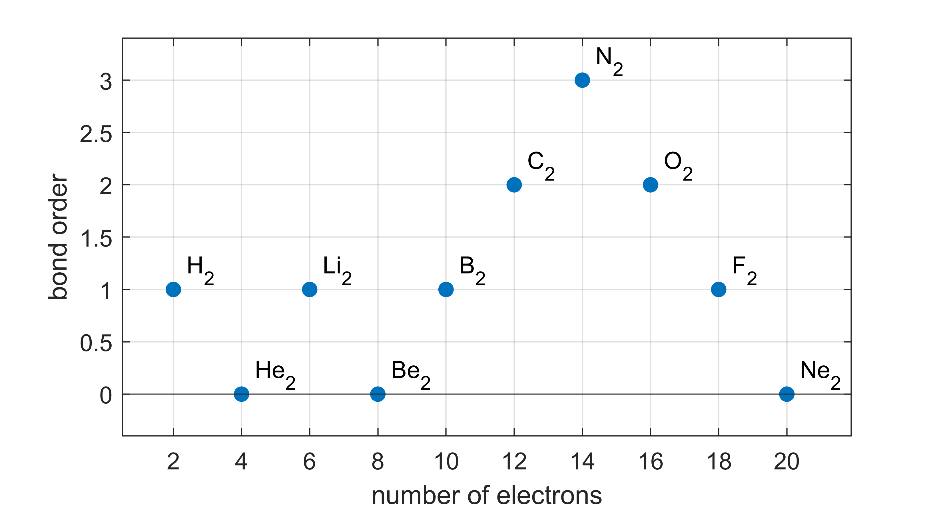
Figure 9.10 The bond orders of the homodiatomic molecules of the first and second row of the periodic table. Note that He₂, Be₂, and Ne₂ have not been observed experimentally.