1. Introduction

Two major theories of physics are Newtonian mechanics and electrodynamics based on Maxwell’s equation. They are able to successfully predict and explain a large number of phenomena observed in the world. However, there exist many phenomena that are not predicted and therefore unexplainable by these theories. Such phenomena are explained by quantum theory, and are therefore called “quantum effects” or “quantum phenomena”. Many of these quantum phenomena are microscopic in origin. The following table lists a few.

Observation	Prediction by classical theory
Atoms and molecules are stable	Atoms are not stable, they collapse.
Discrete emission/absorption spectra	? (no prediction)
Blackbody radiation (sun, fire)	A black body should radiate infinite energy.
Heat capacity goes to zero at 0 K	It should be temperature independent.
Photoelectric effect	Electron emission is intensity dependent.

In the context of chemistry, the first two are particularly important: Quantum theory allows us to understand and predict the stability and the internal structure of atoms and molecules, as well as predict how they interact with light, i.e. their absorption and emission characteristics. For these reasons, quantum theory is foundational to chemistry.

Quantum theory allows us to predict outcomes of experiments on small entities such as atoms and molecules (called quantum systems). However, quantum theory only makes probabilistic predictions about these outcomes, not certain ones. Therefore, at its core, quantum theory is a statistical theory, and it is tested by repeating an experiment many times, or by performing it on many quantum systems at the same time.

1.1. Electromagnetic radiation

Electromagnetic radiation is one of the principal tools for studying the internal structure of atoms and molecules. All processes that generate electromagnetic radiation are quantum processes and cannot be described classically.

Since electromagnetic radiation is so important, we will first examine the two different ways it is modeled in science and engineering: waves and particles.

1.1.1. Wave description

For many large-scale phenomena, it is adequate to model electromagnetic radiation as a traveling wave associated with oscillating electric and magnetic fields that are perpendicular (transverse) to the direction of propagation. This is illustrated in Figure 1.1. The amplitude of the electric and magnetic fields is proportional to the radiation intensity.

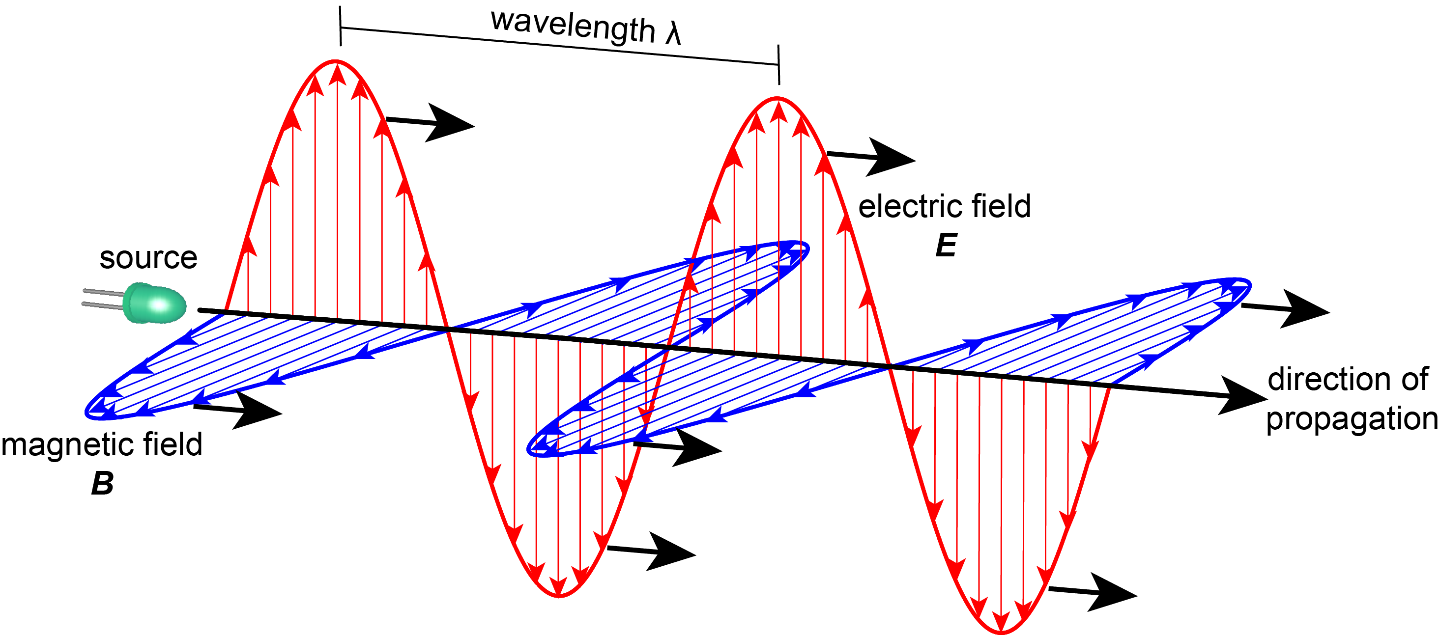
Figure 1.1 The oscillating electric and magnetic fields associated with a traveling plane wave.

The wave travels with a fixed speed that depends on the material it is traveling in. In vacuum, the speed is largest and is 299’792’458 m s^-1. In materials, the wave travels more slowly.

A series of quantities are used to characterize electromagnetic radiation in the wave picture:

• The wavelength \(\lambda\) is the spatial distance between adjacent maxima of the electric (or magnetic) field. It is has dimensions of length, and the SI unit is meters (m). Typical values are 400-750 nm (nanometers) for visible light.

• The wavenumber, indicated by \(\tilde{\nu}\) (Greek letter nu with tilde), is the inverse wavelength: \(\tilde{\nu} = 1/\lambda\). It has dimension of inverse length, and the conventional unit is cm^-1, inverse centimeters.

• The period \(T\) is the time of one oscillation, i.e. the time between two electric-field maxima passing through a fixed point in space. It has dimension of time, and an SI unit of seconds. For example, visible light has a period between 1.5 and 2.5 fs (femtoseconds).

• The frequency \(\nu\) (Greek letter nu) is the inverse of the period, i.e. \(\nu = 1/T\). It is measured in units of Hz (hertz, corresponding to inverse seconds, s^-1). It represents the number of oscillation per second.

• The angular frequency \(\omega\) (Greek letter omega) is related to the ordinary/linear frequency by \(\omega = 2\pi\cdot\nu\). It describes the angle that the oscillation covers if it is considered circular instead of linear. One full oscillation has an angle of \(2\pi\) radians (i.e. 360 degrees). The SI unit for angular frequency is rad s^-1.

The product of the wavelength and the frequency gives the speed of light:

(1.1)\[\lambda\cdot \nu = c\]

Note

Green light has a vacuum wavelength of about 500-550 nm. A wavelength of 500 nm corresponds to a wavenumber of \(20.0\times10^3\) cm^-1, a frequency of 600 THz, a period of 1.67 fs, and an angular frequency of about \(3.77\) rad fs^-1.

1.1.2. Particle description

The second model for electromagnetic radiation is to consider it as a stream of particles. These particles are called photons (a name introduced in 1926 by G. N. Lewis, the chemist after whom Lewis structures of chemical compounds are named). Although already Isaac Newton proposed a particle model for light, it was not until the early twentieth century that it was needed to describe some effects that could not be described using waves. These include the blackbody radiation and the photoelectric effect. The latter was explained by Albert Einstein in 1905 and led to his Nobel Prize 1921.

More precisely, a photon represents the minimum discrete amount (a “quantum”) of energy and momentum that can be transferred from electromagnetic radiation of a specific frequency to matter, or vice versa.

A photon is a “particle” with two special properties: it is mass-less, and it always moves at the speed of light. A photon carries an indivisible quantum of energy. The energy of a photon, \(E_\mathrm{photon}\), relates to wave properties of the associated electromagnetic radiation (frequency, wavelength, etc.):

(1.2)\[E_\mathrm{photon} = h\nu = \hbar\omega = h c/\lambda = h c \tilde{\nu}\]

Energy can be absorbed or emitted by molecules and other materials only in units of the photon energy. A very common unit for photon energy is the electron-volt (eV). One electron-volt is the energy required to move one electron against a potential difference of 1 volt. Its SI value is about \(1.6\cdot10^{-19}\) J - see list of constants.

Note

Radiation of wavelength 500 nm corresponds to a photon energy of \(E_\mathrm{photon} = hc/\lambda = 3.97\times10^{-19}\,\mathrm{J}\), which corresponds to 2.48 eV.

Photons carry momentum. Since they are mass-less, the classical expression \(p=mv\) is not applicable. Instead, the momentum of a photon is

(1.3)\[p = h/\lambda = h\nu/c\]

1.1.3. Wave vs particle

Which of the two models works for describing a particular phenomenon depends on the situations.

• In cases where light/radiation has normal or high intensity, and the materials it interacts with can be treated as homogeneous bulk materials, the wave description works well.

• In contrast, when the light/radiation is very dim, or when it is generated or absorbed by single molecules and other non-classical nano-scale entities, then the particle model is more appropriate.

Note

In X-ray crystallography, crystalline materials are illuminated with X-rays, and the X-ray photons are scattered by the atoms in the crystal. The resulting patterns of diffraction are measured. The photon flux is high, and the interaction between the light/radiation and the crystal can be modeled using waves.

1.1.4. The electromagnetic spectrum

Photon energies, or wavelengths, span many orders of magnitudes. The totality of these possible photon energies or wavelengths is called the electromagnetic spectrum. It is shown in Figure 1.2. It shows both photon energies (particle model) and wavelengths (wave model). The entire spectrum is conventionally subdivided into separate regions with different names. At one end, there are radiowaves, with very low photon energies in the micro-eV range, and wavelengths longer than a meter. At the high-energy end, there are gamma rays, with photon energies of thousands of eVs, and wavelengths in the picometer (pm) range.

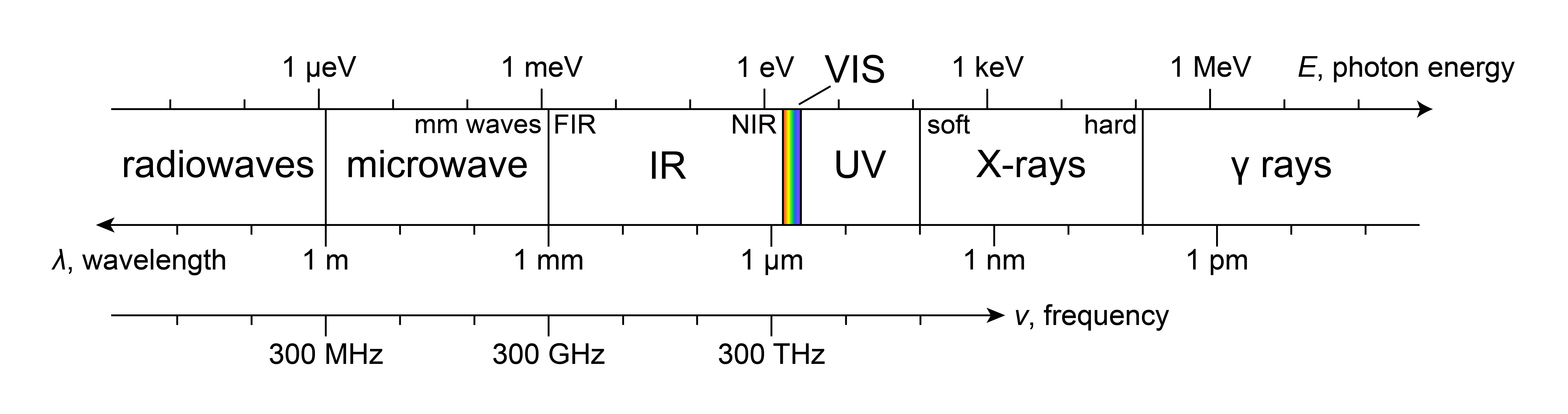
Figure 1.2 The full electromagnetic spectrum, showing wavelengths (wave picture) and photon energies (particle picture).

The human eye is a electromagnetic radiation detector, or photon detector, that is sensitive only over a very narrow range of wavelengths (400-650 nm, corresponding to photon energies of ). This range constitutes the visible spectrum. At the low-energy end, it transitions into the infrared (IR) region, and towards the high-energy end, it goes into the ultraviolet (UV A/B/C, XUV).

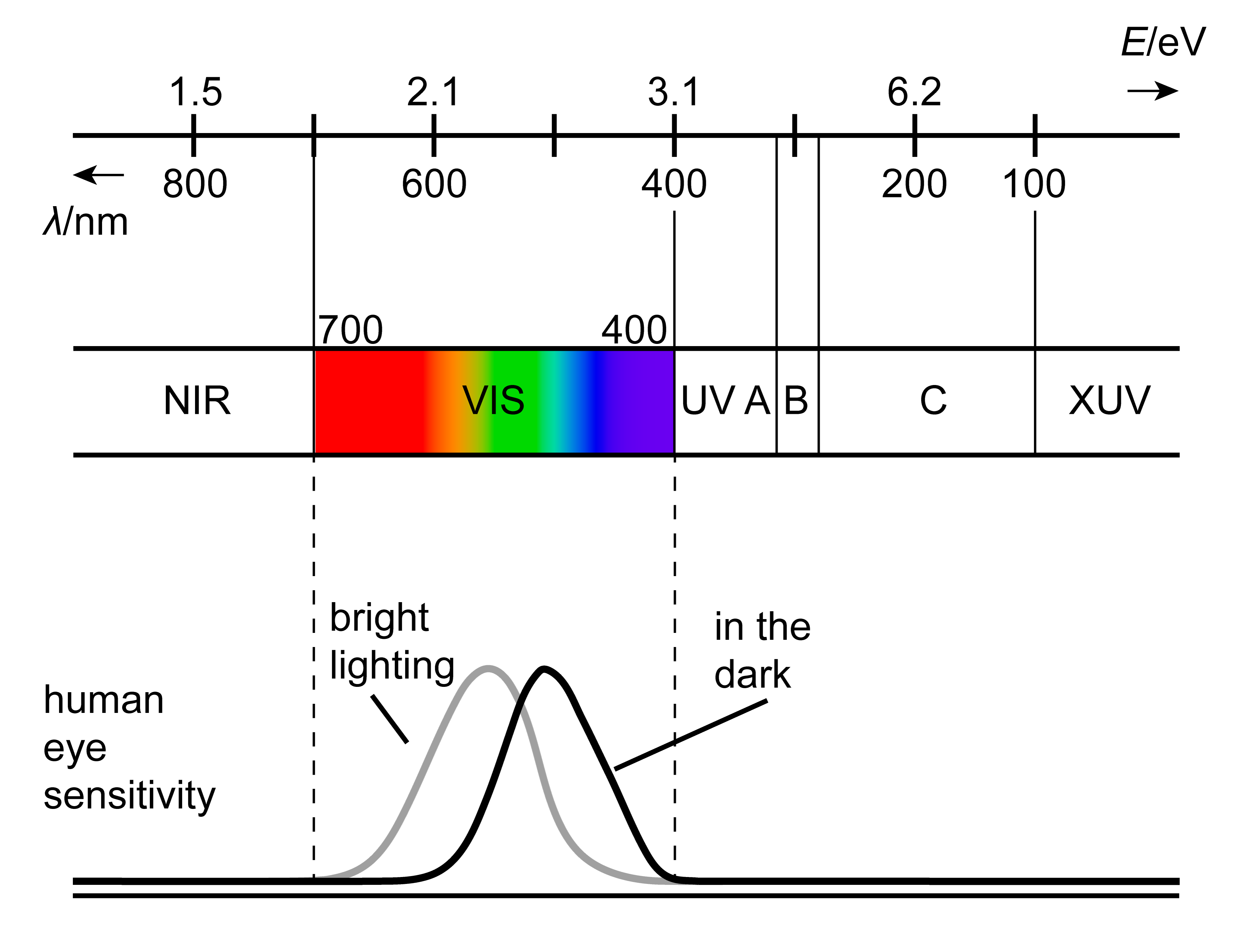
Figure 1.3 The visible part (VIS) of the electromagnetic spectrum, including the sensitivity curves of the human eye under well-lit and dim-lit conditions.

1.2. Absorption and emission

Molecules can absorb and/or emit electromagnetic radiation. There are three basic mechanisms for the interaction between electromagnetic radiation and molecules. These are illustrated in Figure 1.4.

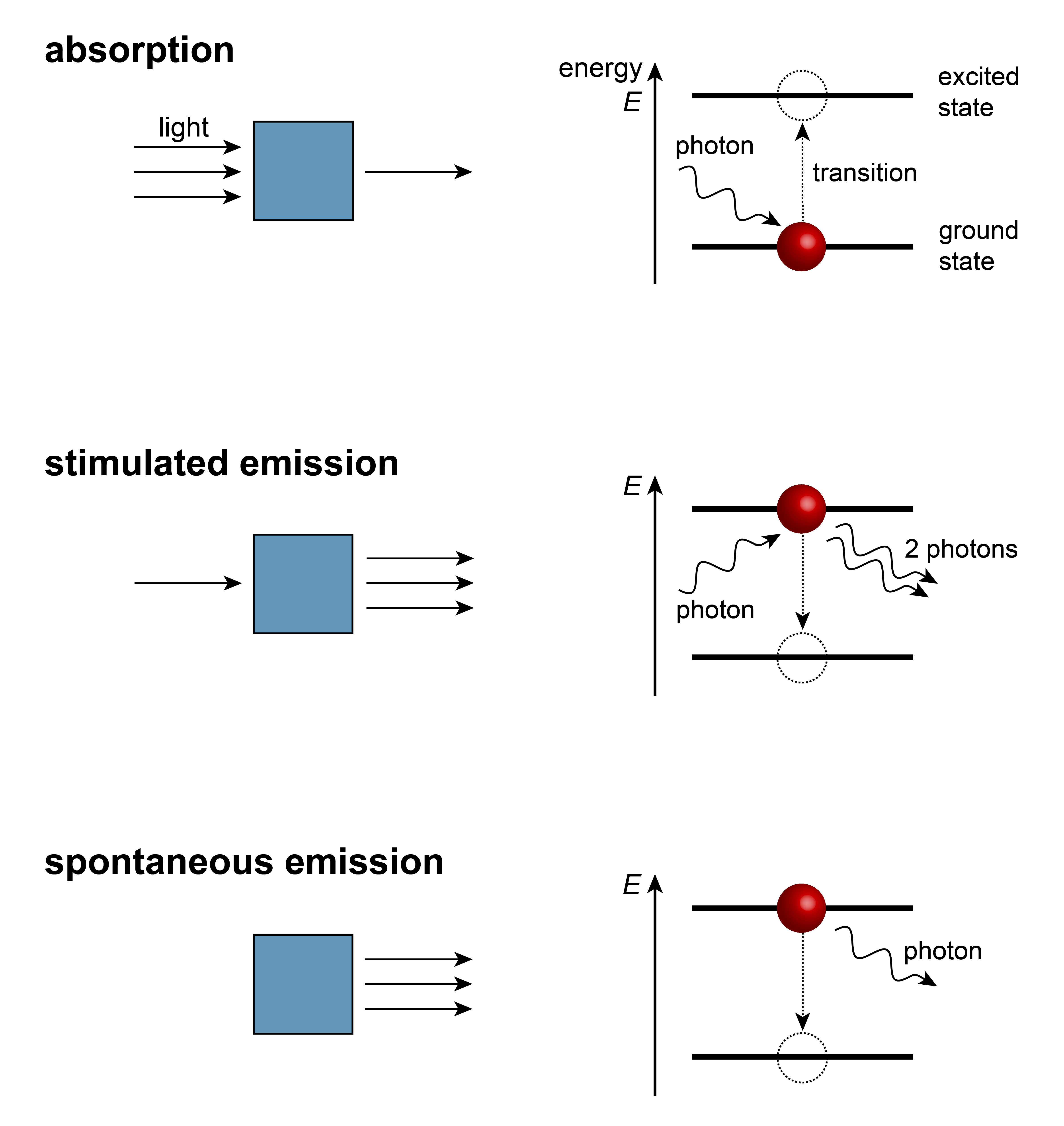
Figure 1.4 Absorption, stimulated emission, spontaneous emission. Left: macroscopic picture, right: energy level diagram.

Absorption of a photon results in the transition of the molecule from its current state (usually its ground state) to a higher-energy excited state. The energy of the photon has to match the difference between the energies of the two states involved:

(1.4)\[\Delta E = E_\mathrm{excited} - E_\mathrm{ground} = E_\mathrm{photon} = h\nu\]

This relation, the requirement that the photon energy match the energy difference, is called the Bohr condition, after Niels Bohr.

Stimulated emission describes a process where one photon interacting with a molecule in an excited state results in two photons emitted. For this process to occur, the energy of the incoming stimulating photon must match the energy difference.

Spontaneous emission describes the situation where a molecule in an excited state emits a photon directly, without a stimulating photon. This process is called spontaneous, but it is actually stimulated by vacuum field fluctuations. The rate of spontaneous emission is strongly frequency-dependent: it scales with the cube of the frequency. For low-frequency radiation (such as radiofrequency or microwaves), it is negligibly slow. For higher frequencies (visible, ultraviolet), it is very fast.

Both forms of emission, stimulated and spontaneous, are forms of radiative decay.

There are many different sources of electromagnetic radiation. The strongest natural visible-light source is the sun. It emits so-called black-body radiation, with most intensity in the UV, visible, and IR regions. Figure 1.5 shows the solar emission spectrum, as seen above the atmosphere and on the surface of the earth. The difference between the two spectra is due to the absorption of sunlight by atmospheric molecules such as water and carbon dioxide.

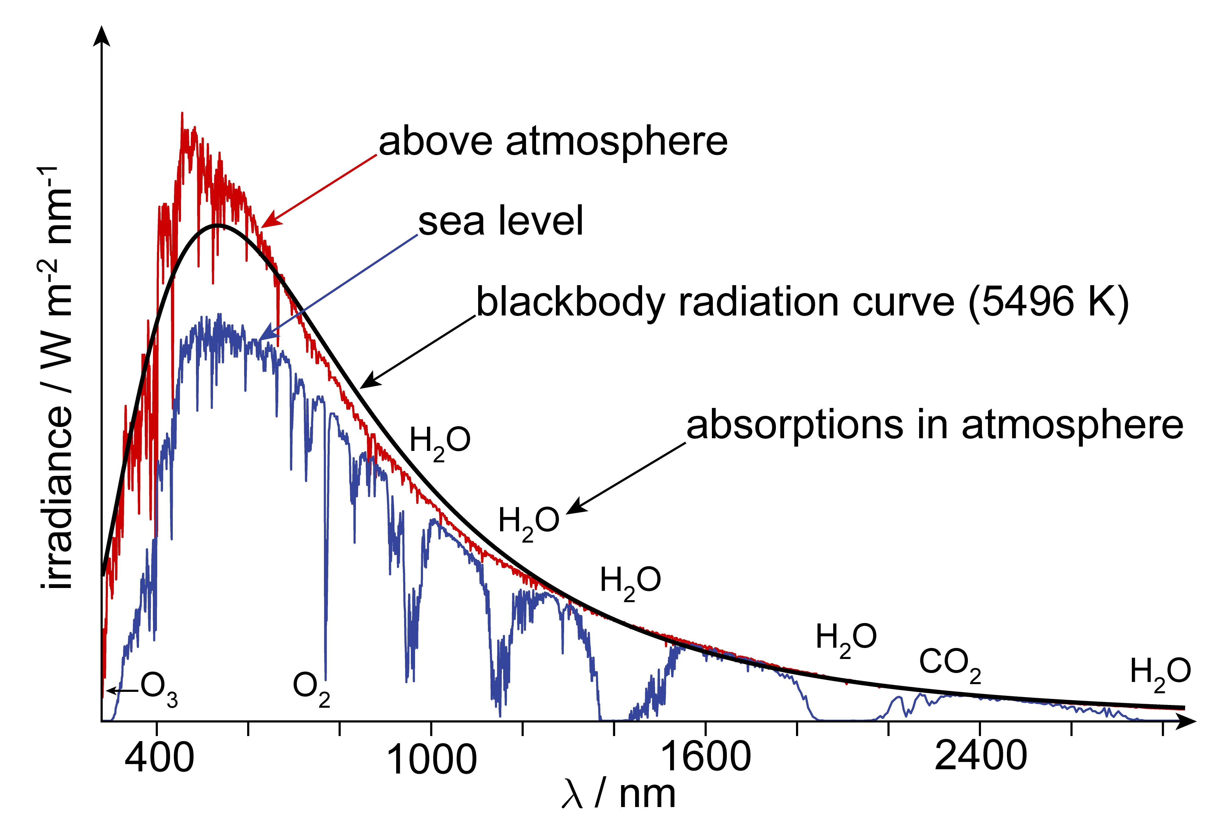
Figure 1.5 The emission spectrum of the sun, both above the atmosphere and on the surface of the earth. The black curve indicates the predicted emission spectrum of a black body at a temperature of 5496 K.

The intensity of black-body radiation as a function of wavelength is given by Planck’s law

(1.5)\[B_\lambda(\lambda,T) = 2hc^2 \frac{\lambda^{-5}}{ \mathrm{e}^{hc/(\lambda k_\mathrm{B}T)} -1 }\]

Luminescence is the property of a material to emit light upon stimulation (except by heating, which is the black-body radiation discussed above). It is categorized based on the type of process that promotes the molecule into the excited state, such that it can emit light. Types of luminescence include photoluminescence (fluorescence and phosphorescence), chemiluminescence (bioluminescence etc), electroluminescence, mechanoluminescence, and thermoluminescence (which is distinct from black-body radiation).

1.3. Beer-Lambert law

When radiation of a given frequency/wavelength hits an absorbing molecule, it is not possible to predict with certainty whether a specific molecule will absorb a photon or not in a given time interval. However, quantum theory can predict the probability for this absorption event. This means that it is possible to predict what is happening in the presence of a large number of molecules: When the radiation passes through a medium containing many molecules (see Figure 1.6), the probabilistic absorption by each molecule results in the overall attenuation of the incident beam by the medium.

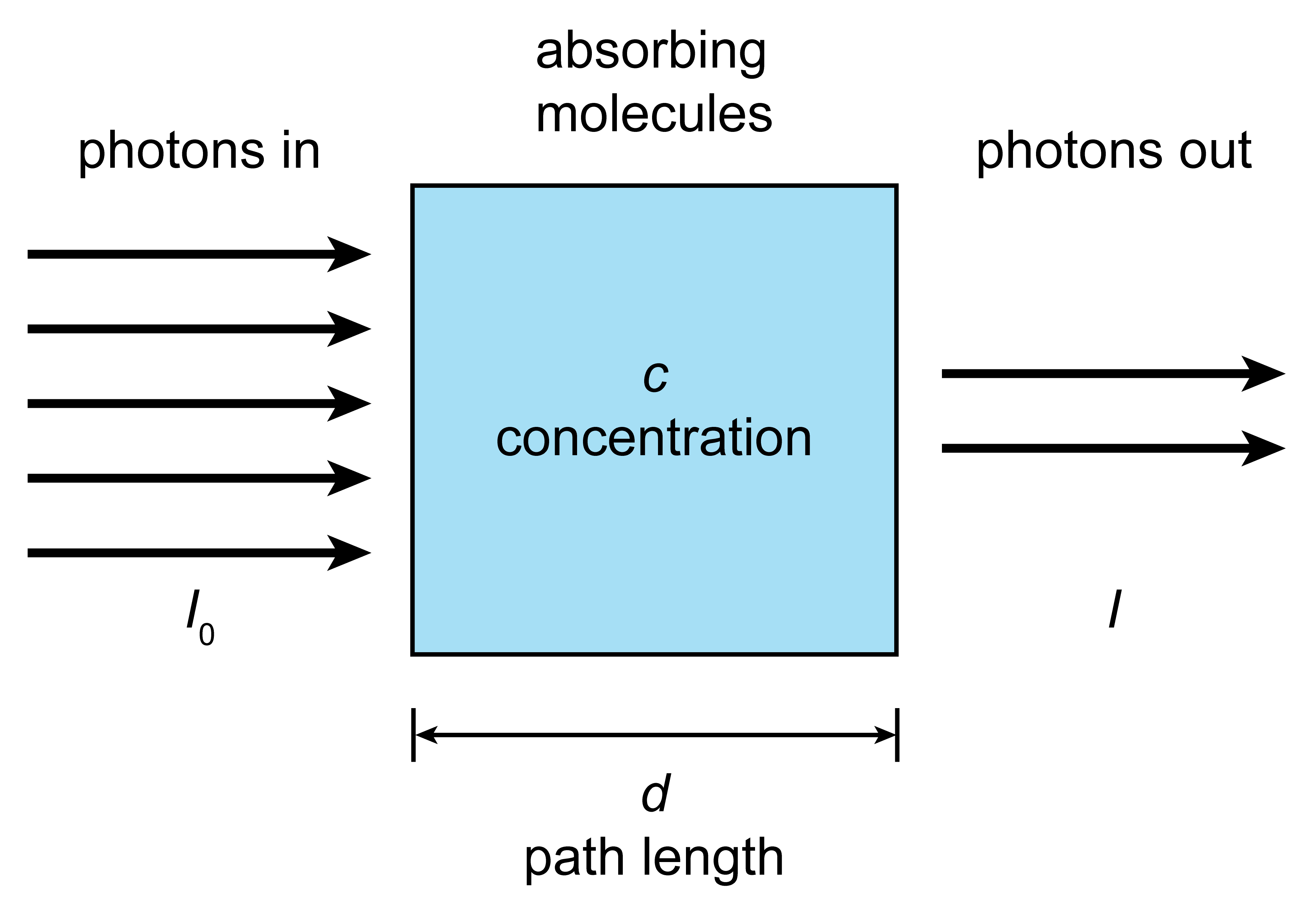
Figure 1.6 Attenuation (or extinction) of a light beam traveling through an absorbing medium.

The expected number of absorbed photons is given by the following exponentially decaying function

(1.6)\[I(\lambda) = I_0 \cdot \mathrm{exp}[-\sigma(\lambda) n d]\]

where \(I_0\) is the incident intensity, i.e. the number of photons per time per area (radiant flux density) and \(I\) is the exiting light intensity, i.e. the number of photons per time per area that are not absorbed. \(\sigma(\lambda)\) is the wavelength-dependent absorption cross section, \(n\) is the number concentration (molecules per volume), and \(d\) is the path length.

An important quantity in this context is the transmittance, defined as

(1.7)\[T(\lambda) = \frac{I(\lambda)}{I_0}\]

\(T\) is dimension-less and can assume values between 0 and 1. A transmittance of 0 indicates that the medium completely absorbs the light, and a transmittance of 1 indicates that nothing at all is absorbed at wavelength \(\lambda\).

Another practically very important quantity relating incident and exiting intensity is the absorbance, defined as the negative base-10 logarithm of the transmittance,

(1.8)\[A(\lambda) = -\mathrm{log}_{10}T(\lambda)\]

With this, the exponential law for the attenuation of radiation going through an absorbing medium becomes the Beer-Lambert law, Eq. (1.9)

(1.9)\[A(\lambda) = \epsilon(\lambda) c d\]

where \(\epsilon = \sigma N_\mathrm{A} / \mathrm{log}(10)\), with Avogadro’s number \(N_\mathrm{A}\), is called the molar absorption coefficient (or molar extinction coefficient). Conventional units for the path length are cm, for the concentration M ( = mol L^-1), so that the conventional unit for \(\epsilon\) is M^-1 cm^-1.

Note

It is useful to be familiar with numerical values of transmittance and absorbance. Here are a few examples:

• \(A = 0.1\) means \(T = I/I_0 = 0.8\), indicating that about 80% of the radiation is transmitted, the remaining 20% absorbed.

• \(A = 1\) means \(T = I/I_0 = 0.1\), indicating 10% transmission and 90% absorption.

• \(A = 2\) gives \(T = I/I_0 = 0.01\) and corresponds to 1% transmission and 99% absorption.

In practice, concentrations and path lengths are always adjusted to assure that \(A<1\). The reason is that higher absorbances can only be reached with high concentrations, which introduce non-linear effects that result in deviations from the Beer-Lambert law.

The molar absorption coefficient is a property of the medium and is wavelength dependent, \(\epsilon(\lambda)\). A plot of \(T\), \(A\), or \(\epsilon\) as a function of wavelength or frequency is called a spectrum. Figure 1.7 shows an example.

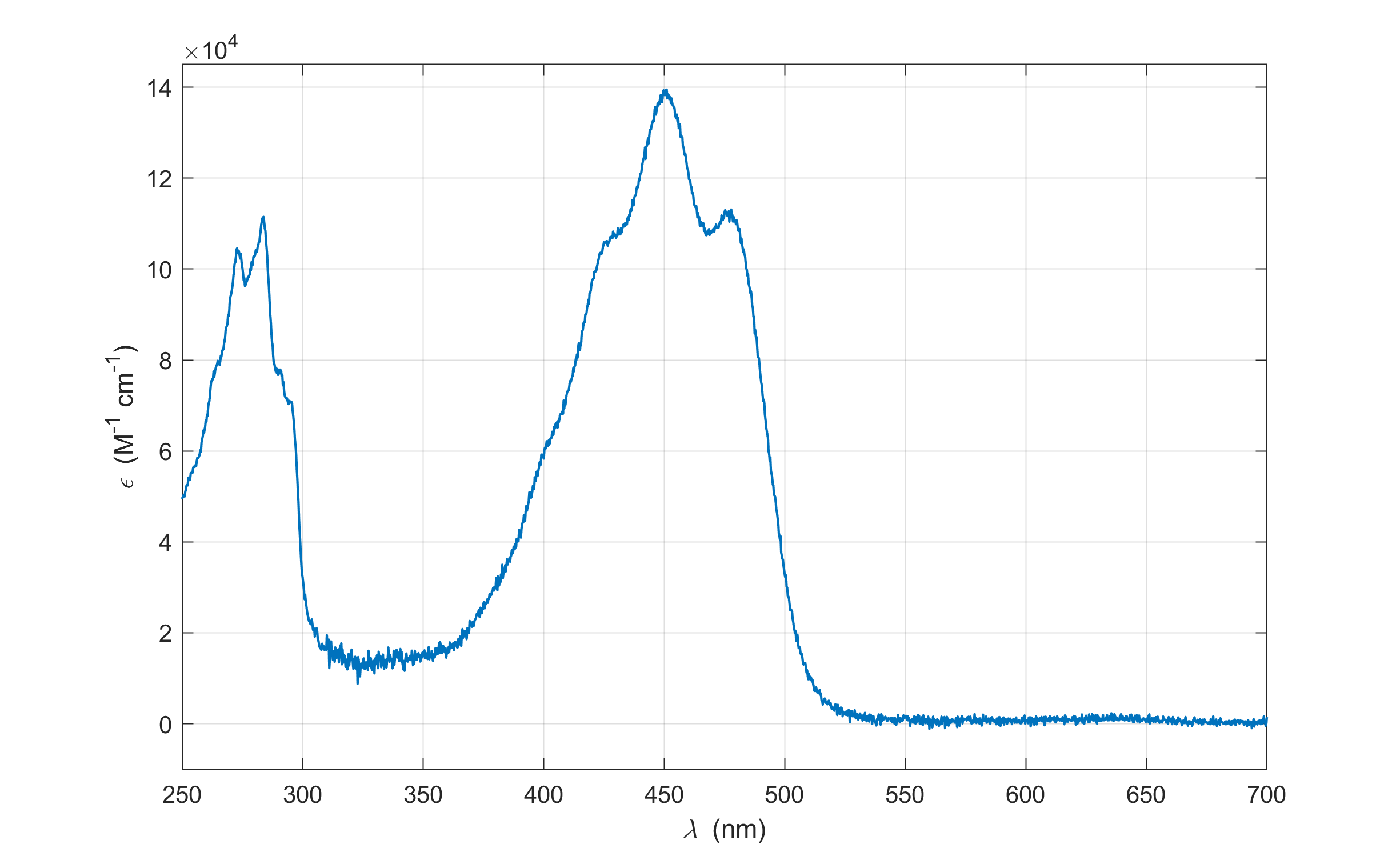
Figure 1.7 The absorption spectrum of beta-carotene in hexane, plotted as molar absorption coefficient as a function of wavelength. There is a strong absorption maximum at about 400 nm, with a corresponding \(\epsilon\) of about \(1.4\times10^{5}\,\mathrm{M}^{-1}\mathrm{cm}^{-1}\).

1.4. Matter waves

Streams of moving massive particles (such as electron and neutrons) can be modeled as traveling waves. The associated wavelength is

(1.10)\[\lambda_\mathrm{dB} = \frac{h}{p} = \frac{h}{m v} = \frac{h}{\sqrt{2m E_\mathrm{kin}}}\]

where \(m\) is the mass of the particles, \(v\) is their speed, and \(E_\mathrm{kin}\) their kinetic energy. (This expression is valid as long as \(v\) is much smaller than the speed of light, otherwise a correction based on the theory of relativity has to be included.)

The wavelength \(\lambda_\mathrm{dB}\) is called the de Broglie wavelength. The concept of modeling massive particles using a wave model was initially proposed theoretically by Louis de Broglie in 1923/24, and has then been first experimentally observed for the diffraction of electrons. Nowadays, it is routinely used in the description and analysis of electron and neutron diffraction experiments.

Note

Electron diffraction is a method where a beam of electrons (mass \(m_\mathrm{e}\)) with high kinetic energy is aimed at a crystalline sample, and the electrons are diffracted in a wave-like fashion. The wavelength associated with the electrons in the beam can be calculated using the de Broglie relationship. For examples, electrons accelerated by a voltage of 1.2 kV have a kinetic energy of 1.2 keV and a wavelength of

(1.11)\[\lambda = \frac{h}{\sqrt{2m_\mathrm{e}E_\mathrm{kin}}} = 35\,\mathrm{pm}\]

1.5. The hydrogen atom

A hydrogen atom consists of a proton and an electron. Classical electromagnetic theory based on Maxwell’s equations predicts that a charge emits radiation whenever it is accelerated perpendicular to its direction of motion. (This effect is utilized in synchrotrons and free-electron lasers to generate high-energy radiation). For a hydrogen atom, where the electron is orbiting the nucleus, it predicts that the electron will radiate energy, slow down, and eventually collapse into the nucleus (see Figure 1.8). The atom ceases to exist. Therefore, pre-quantum physics is unable to explain the stability of the hydrogen atom, nor of any other atom.

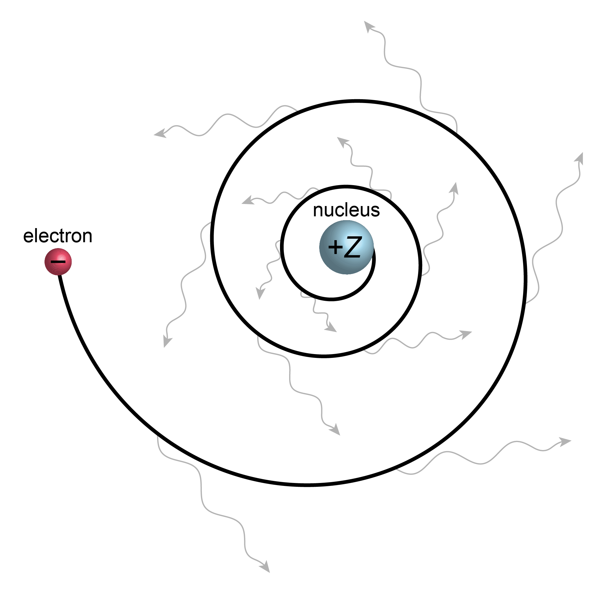
Figure 1.8 The classical picture of a hydrogen atom. The moving electron is accelerated perpendicular to its direction of motion, therefore emits radiation, loses energy, and collapses into the nucleus.

The first successful model of the hydrogen atom is due to Niels Bohr. In this model, the electron is assumed to orbit around the nucleus in a circular orbital motion without radiating. For such an orbit to be stable, the centripetal electrostatic attraction force between the electron and the nucleus has to be opposite and equal in magnitude to the centrifugal force experienced by the electron:

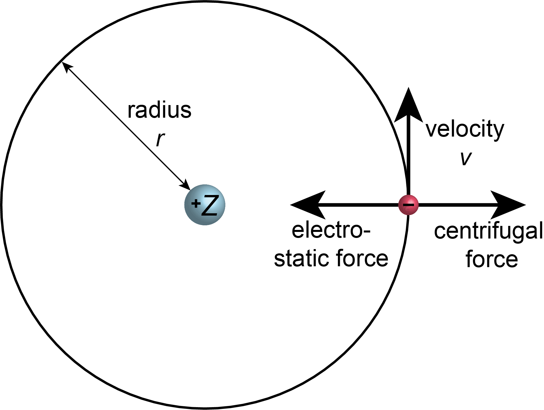
Figure 1.9 For a stationary orbit, the centripetal electrostatic force on the electron has to be opposite and equal in magnitude to the centrifugal force.

(1.12)\[\frac{1}{4\pi\epsilon_0}\frac{Ze^2}{r^2} = \frac{m_\mathrm{e}v^2}{r}\]

\(Z\) is the dimensionless nuclear charge number (1 for hydrogen/proton, 2 for helium nucleus, 3 for lithium nucleus, etc.), \(\epsilon_0\) is the electric constant (also called vacuum permittivity), \(e\) is the (positive) elementary charge, \(m_\mathrm{e}\) is the mass of the electron, and \(v\) is the speed of the electron.

In order to match experiments, Bohr postulated that within this model only certain values of angular momentum \(l\) of the electron are “allowed”: \(l = m_\mathrm{e}vr = n\hbar\), where \(n\) is an positive integer (1, 2, 3, etc). They are allowed in the sense that only with these values the electrons will be in a stable stationary orbit. This ad-hoc assumption is justified only by its eventual success in reproducing experimentally observed emission and absorption lines of hydrogen atoms. This condition yields for the speed:

(1.13)\[v = \frac{n\hbar}{m_\mathrm{e}r}\]

Inserting this back into the right-hand side of the equality of forces gives

(1.14)\[\frac{1}{4\pi\epsilon_0}\frac{Ze^2}{r^2} = \frac{m_\mathrm{e}n^2\hbar^2}{m_\mathrm{e}^2r^3} = \frac{n^2\hbar^2}{m_\mathrm{e}r^3}\]

This can be rearranged to give an expression for the allowed values for \(r\)

(1.15)\[r = 4\pi\epsilon_0\frac{\hbar^2}{m_\mathrm{e}e^2}\cdot\frac{n^2}{Z} = a_\mathrm{0}\cdot\frac{n^2}{Z}\]

The quantity \(a_0\) has dimensions of length and is called the Bohr radius. Its value is \(a_0\approx 52.9\) pm. This equation indicates that, within this model, only certain radii would be “allowed” for the electron orbits, depending on the integer \(n\), which is called a quantum number. The radius of the electron orbits grow quadratically with \(n\) and is inversely proportional to the nuclear charge, \(Z\).

The total energy of the electron \(E\) in this model is the sum of its kinetic energy and its potential energy:

(1.16)\[E = \frac{1}{2}m_\mathrm{e}v^2 - \frac{1}{4\pi\epsilon_0}\frac{Ze^2}{r}\]

Rearranging the force balance equation to get an expression for \(m_\mathrm{e}v^2\) and inserting that into the expression for \(E\) gives

(1.17)\[E = -\frac{e^2}{8\pi\epsilon_0a_0}\cdot\frac{Z^2}{n^2} = -hcR_\infty \frac{Z^2}{n^2} = - 13.606\,\mathrm{eV}\cdot\frac{Z^2}{n^2}\]

The quantity \(R_\mathrm{\infty}\) is the Rydberg constant. It has dimension of inverse length, and its value is about 109373 cm^-1. This expression shows that the energies of the electron (and therefore the overall hydrogen atom) are discrete, they are said to be “quantized”. All energies are negative. Energy zero is obtained if the electron is infinitely far from proton (potential energy zero) and at rest (kinetic energy zero).

The allowed energy states of the hydrogen atom are plotted in Figure 1.10. A transition of the hydrogen atom from an initial state with quantum number \(n_\mathrm{i}\) to a final state with quantum number \(n_\mathrm{f}\) results in a decrease or increase of the energy by

(1.18)\[\Delta E = E_{n_\mathrm{f}} - E_{n_\mathrm{i}} = h c R_\infty Z^2\left(\frac{1}{n_\mathrm{i}^2}-\frac{1}{n_\mathrm{f}^2}\right)\]

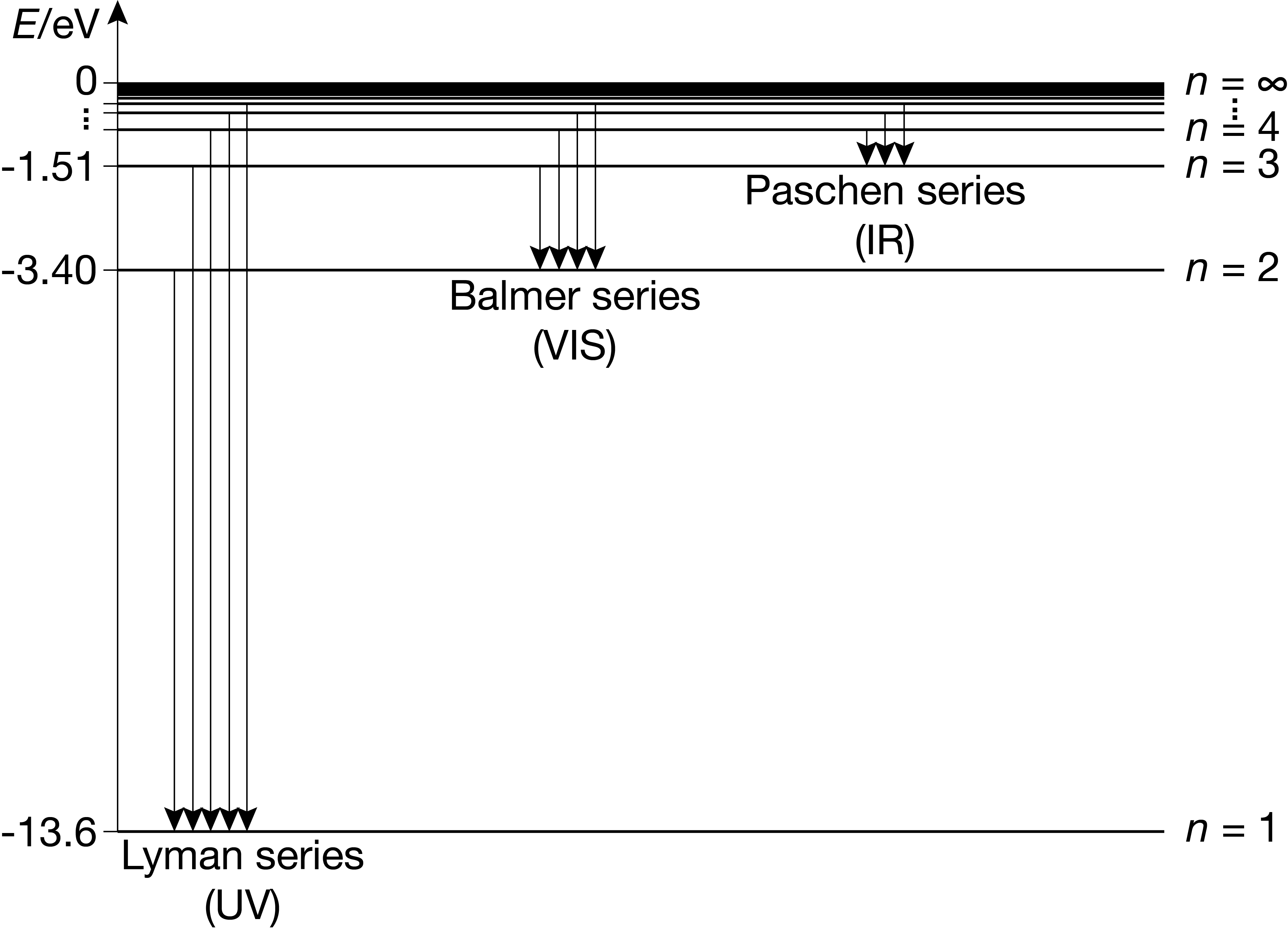
Figure 1.10 The stationary states of a hydrogen atom, including energies, quantum numbers, and the emissive transitions of the Lyman, Balmer, and Paschen series.

This equation describes transitions between bound states, i.e. states where the electron is bound to the nucleus. For an emissive transition (\(\Delta E\)), the internal energy decreases, with the excess energy discharged by emitting a photon. For an absorptive transition (\(\Delta E >0\)), the internal energy increases, with the additional energy coming from an absorbed photon. When a photon with 13.6 eV or more of energy is absorbed by a hydrogen atom in its ground state, the electron is ejected from the atom. Therefore, this is the ionization energy of the hydrogen atom. The excess energy above 13.6 eV is carried away as kinetic energy of the emitted electron. Such states are called unbound states, and there are no limitations on the energy - they form a continuum.

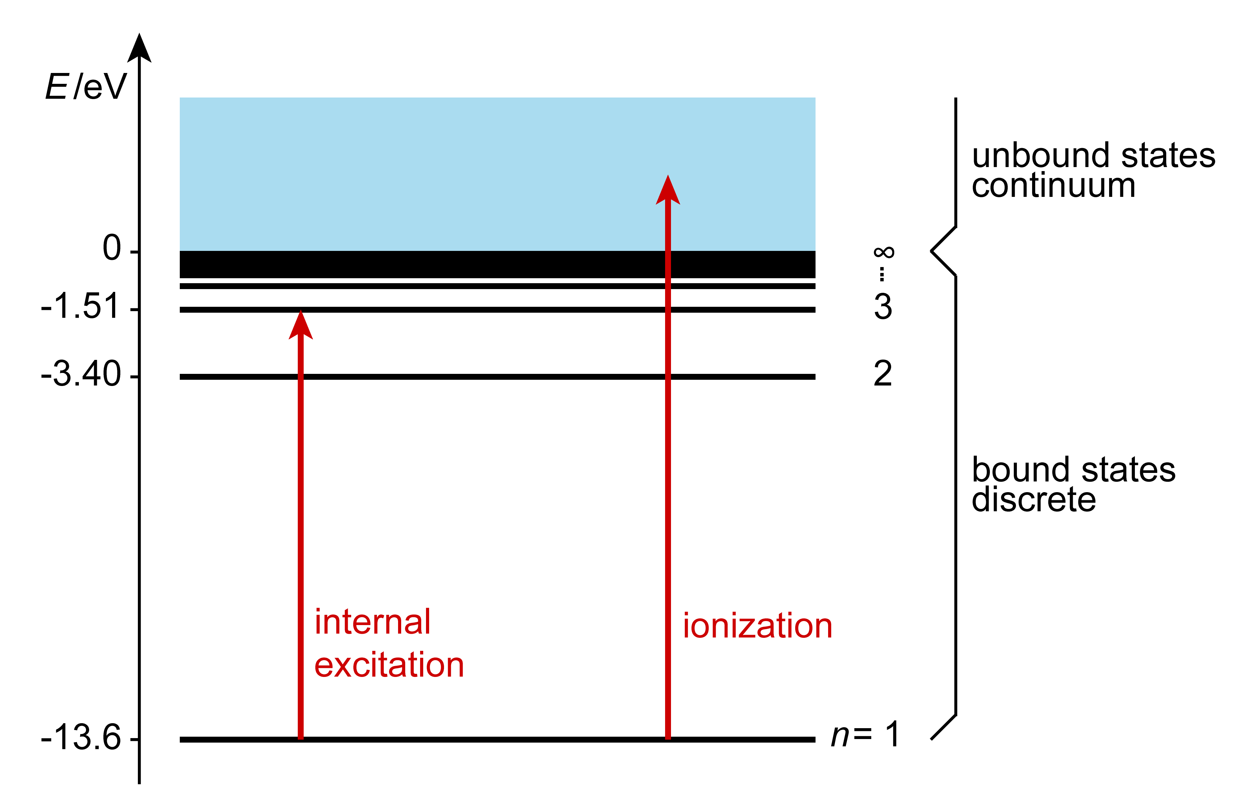
Figure 1.11 The distinction between bound and unbound states of the hydrogen atom.

The Bohr model correctly predicts the energy levels of the hydrogen atom, and therefore the energies and wavelengths of the lines in its emission spectrum. However, it fails to predict the emission lines of atoms or ions with more than one electron. Also, the Bohr model’s assumption of an orbital angular momentum of \(l=n\hbar\) is incorrect already for the ground state (\(n=1\)), since it is known from experiment that the electron in the hydrogen atom does not have an orbital angular momentum (i.e. it has \(l=0\))! The Bohr model was soon superseded by quantum theory.

1.6. The Boltzmann distribution

In an ensemble of identical atoms or molecules at thermal equilibrium with their surroundings, different atoms/molecules can occupy different states. The number of atoms/molecules in the ensemble occupying a specific state with energy \(E_j\) is proportional to an energy- and temperature-dependent exponential factor:

(1.19)\[\mathrm{e}^{-E_j/k_\mathrm{B}T}\]

where \(T\) is the absolute temperature (in kelvin, K), and \(k_\mathrm{B}\) is the Boltzmann constant (in joules per kelvin, J K^-1). The associated distribution of occupancies across states is called the Boltzmann distribution. The expression indicates that states with higher energies are exponentially less occupied.

Two or more states that have the same energy are said to be degenerate. Together, they form one energy level. The multiplicty \(g\) captures the number of degenerate states. For example, \(g=2\) indicates a multiplicty of two, ie. two degenerate states. The concept is illustrated in Figure 1.12.

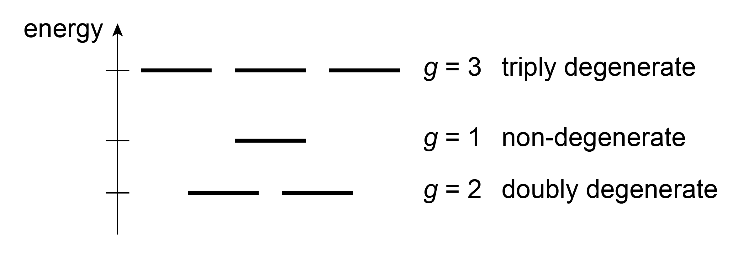
Figure 1.12 The concept of degeneracy. Each horizontal line represents one state. States are called degenerate if they have the same energy. The multiplicity of an energy level, \(g\), equals the number of states with that energy.

For two energy levels \(i\) and \(j\) with energies \(E_i\) and \(E_j\) and degeneracies \(g_i\) and \(g_j\), the Boltzmann distribution gives

(1.20)\[\frac{N_i}{N_j} = \frac{g_i \mathrm{e}^{-E_i/k_\mathrm{B}T}}{g_j \mathrm{e}^{-E_j/k_\mathrm{B}T}} = \frac{g_i}{g_j}\mathrm{e}^{-(E_i-E_j)/k_\mathrm{B}T}\]

Here, \(N_i\) is the total population of all degenerate states with energy \(E_i\), and \(N_j\) is defined analogously.

Figure 1.13 illustrates the Boltzmann distribution for a simple system with two state, a ground state indicated by 1 and an higher-energy excited state indicated by 2. It shows the ratio of populations, \(N_2/N_1\), as a function of temperature. When the energy difference between the two states, \(\Delta E = E_2-E_1\), is much smaller than the thermal energy, \(k_\mathrm{B}T\), then both states are almost equally populated (left side in the figure). This is the high-temperature regime. In the opposite situation, when the energy difference is much larger than the thermal energy, we are in the low-temperature regime, and only the lower state is significantly populated (right side in the figure).

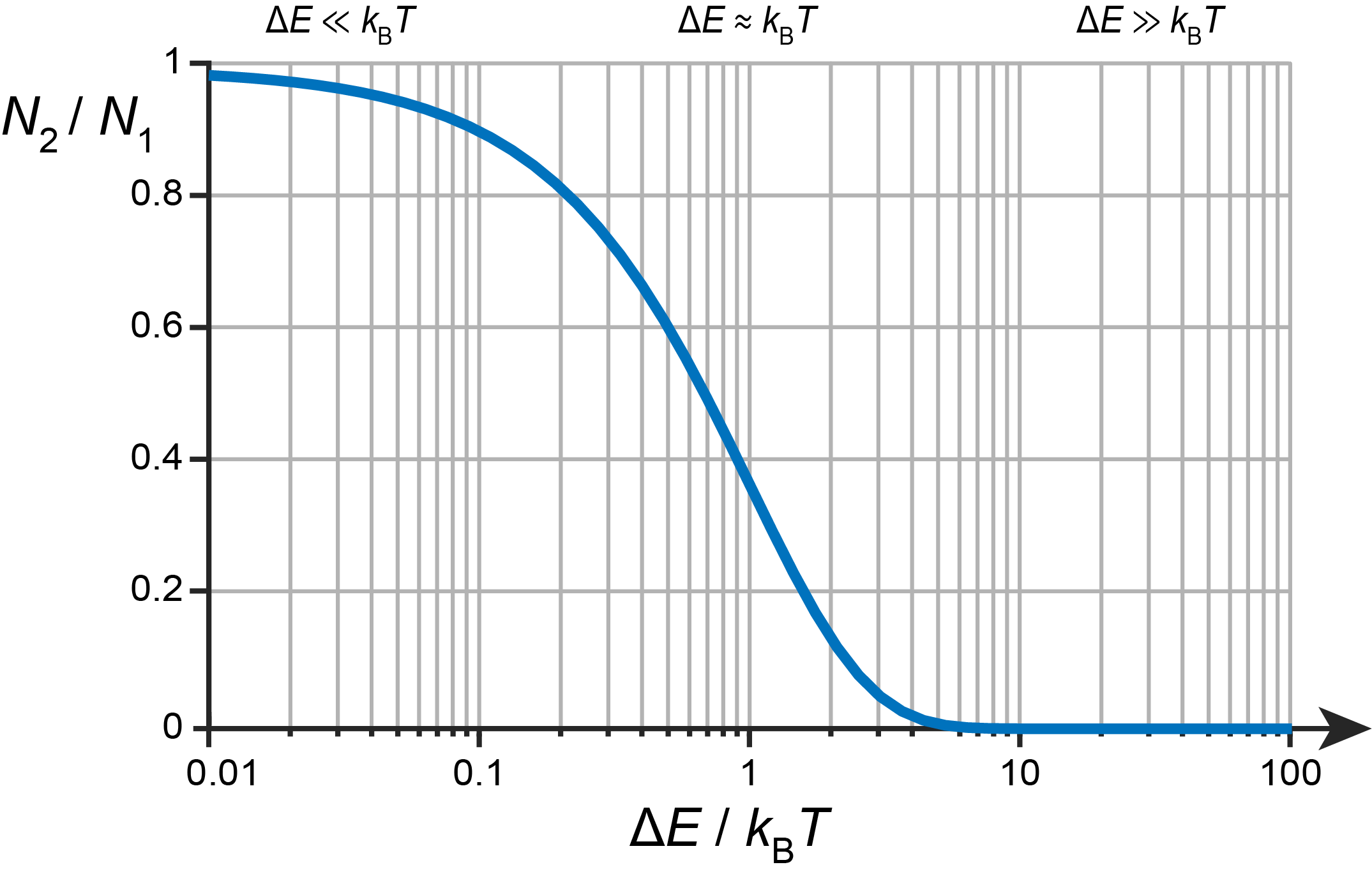
Figure 1.13 The dependence of the population ratio \(N_2/N_1\) on the energy difference \(\Delta E = E_2-E_1\) and temperature \(T\) for a two-level system. Note the logarithmic scale on the horizontal axis.

Note

The first set of excited states of the hydrogen is about 10.2 eV above the non-degenerate ground state and is 4-fold degenerate (\(\Delta E = 10.2\,\mathrm{eV}\), \(g_1 = 1\), \(g_2=4\)). In a large ensemble of hydrogen atoms at a high temperature of 1000 K, the ratio of populations is therefore

(1.21)\[\frac{N_2}{N_1} = \frac{4}{1}\mathrm{e}^{-\frac{\Delta E}{k_\mathrm{B}T}} \approx 1.6\cdot 10^{-51}\]

This means that essentially all hydrogen atoms are in the ground state. This is a consequence of \(\Delta E\gg k_\mathrm{B}T\) in this case.

The first excited vibrational state of diiodine, I₂, is 26.6 meV above the ground state. Both states are non-degenerate (multiplicity is 1). At room temperature (298 K), the population ratio is \(N_2/N_1 = 0.355\). In this case, \(\Delta E\approx k_\mathrm{B}T\), and a significant fraction of the molecules is in the excited state.