2. Quantum theory

This chapter lays out the theoretical foundation of quantum theory, as needed for understanding atoms, molecules, and spectroscopy. Quantum theory makes predictions about the outcomes of measurements on microscopic systems such as atoms and molecules. It is able to predict possible outcomes and their probabilities, but it is not able to predict which of the possible outcomes will be observed in a given single experiment. These outcomes are currently unpredictable and appear random. Despite this apparent incompleteness, however, quantum theory is immensely useful. The reason for this is that we rarely have situations where only single outcomes are observed or utilized. This is especially true in chemistry and material science, where we rarely look at single atoms, molecules, or photons at a time, but rather at very large numbers of them at once.

Note

Large numbers: 1 mL of a 1 mM solution contains \(6\times10^{17}\) molecules. A 532 nm laser pulse with 1 mJ energy contains almost \(3\times10^{15}\) photons.

The collection of particles whose behavior or experimental response we are interested in predicting using quantum theory is called the quantum system. In quantum chemistry, the quantum systems are predominantly atoms, molecules, and solid-state materials. They are described either as a collection of atoms if the purpose is to describe vibrations and molecular rotation, or as electrons moving in an environment of fixed nuclei if the purpose is to model the electronic structure and chemical reactivity.

The essential elements of quantum theory are summarized in just five postulates, statements that build the foundation of the theory. These postulates cannot be derived from any more fundamental principles, but they have been proven valid as all predictions made by the theory built on them are consistent with experimental results. They are listed in Figure 2.1.

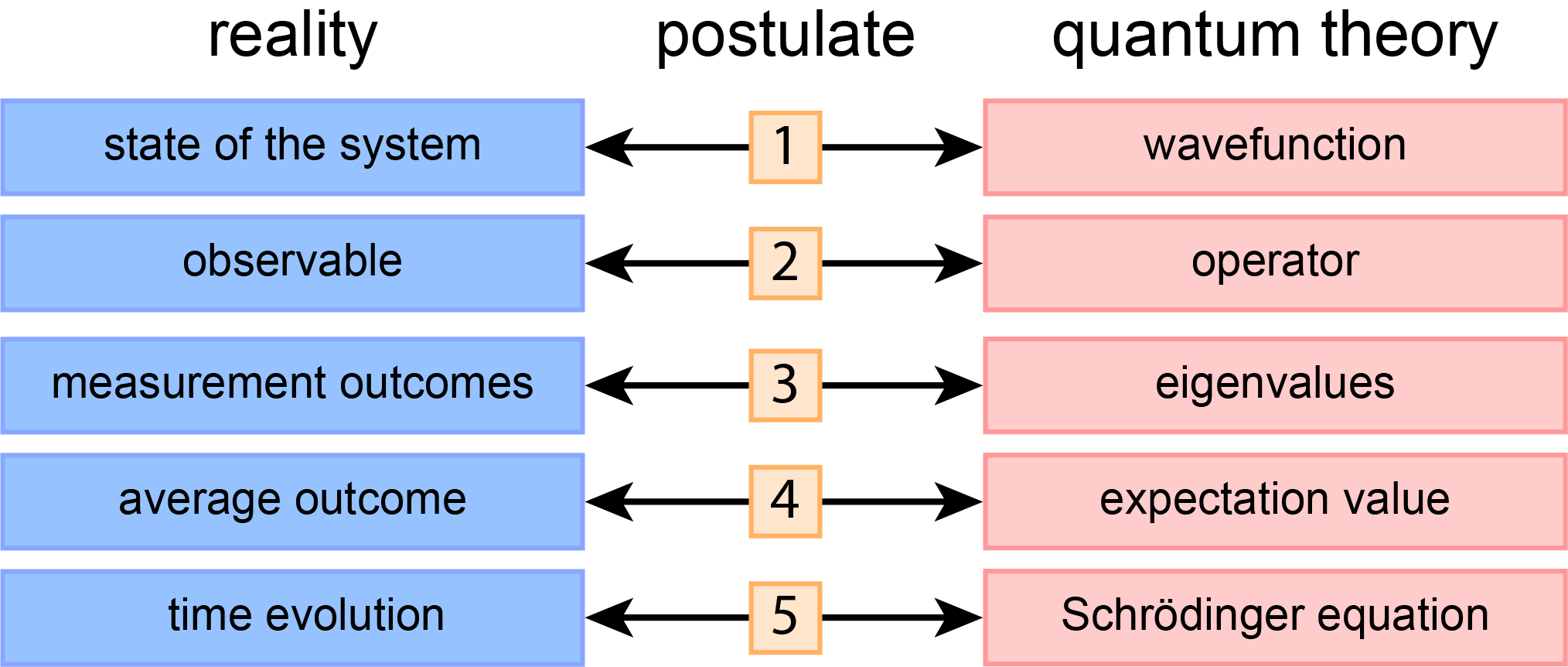
_images/theory_postulates.png — Figure 2.1 The five fundamental postulates of quantum theory.

Each of the five postulates introduces a mathematical entity that is used to represent an element of reality. According to postulate 1, in quantum theory the state of a system is represented by a wavefunction. Postulates 2, 3, and 4 relate to how observables are represented by operators and how measurement outcomes are predicted. Finally, postulate 5 gives the Schrödinger equation, which describes how a wavefunction changes with time.

In the rest of this chapter, we discuss each of the five postulate in turn and introduce the associated mathematical concepts. The postulates will be applied in subsequent chapters.

2.1. Wavefunctions and states

Postulate 1 states that in quantum theory, a state of a system of particles is mathematically represented by a wavefunction, usually denoted by \(\varPsi\). Different states of the system are represented by different wavefunctions. A wavefunction is a scalar function, i.e. it returns a single number, but this number can be complex-valued. It is a function of the positions of all particles and depends on time:

(2.1)\[\varPsi(x_1,y_1,z_1,x_2,y_2,z_2,\dots,x_N,y_N,z_N,t)\]

where \(x_i\), \(y_i\), and \(z_i\) indicate the position of particle \(i\), \(t\) indicates time, and \(N\) is the number of particles. For a single particle moving in 3D space, the wavefunction depends on three position coordinates and time, \(\varPsi(x,y,z,t)\). Often, we will consider a single particle that can move only along one dimension (1D). A wavefunction for such a particle is written as \(\varPsi(x,t)\), where \(x\) is the position of the particle. Many of the equations generalize easily to more than one dimension and more than one particle.

If a particle has spin, such as the electron or the proton, the spin coordinate \(m\) is added as the fourth coordinate. A wavefunction for one electron moving in three dimensions would be \(\varPsi(x,y,z,m,t)\). Unlike the spatial coordinates, which can assume any value (they are continuous), the spin coordinate \(m\) is discrete. For an electron or other particle of spin 1/2, the only possible values for \(m\) are \(+1/2\) and \(-1/2\).

A wavefunction is a mathematical tool to calculate probabilities. For one particle moving along one dimension, the probability of finding it between \(x\) and \(x+\mathrm{d}x\) is given by \(\varPsi(x,t)^*\varPsi(x,t)\mathrm{d}x\), where \(^*\) indicates the complex conjugate. The quantity

(2.2)\[\varPsi^*\cdot\varPsi = |\varPsi|^2\]

is the probability density, i.e. the probability per unit length of finding the particle in the immediate vicinity of \(x\). Whereas \(\varPsi\) is an auxiliary quantity, \(|\varPsi|^2\) has direct physical meaning. This interpretation of \(\varPsi\) in terms of a probability is called the Born rule, after Max Born.

We will restrict ourselves to a special class of states, those that are described by wavefunctions that are simple products of two factors

(2.3)\[\varPsi(x,t) = \psi(x)\cdot \mathrm{e}^{\mathrm{i}\omega t}\]

where the first factor \(\psi(x)\) is the spatial wavefunction, and the second factor \(\mathrm{e}^{\mathrm{i}\omega t}\) captures all of the time dependence (\(\omega\) is an angular frequency). For states with this form of wavefunction, the associated probability density is independent of time, \(|\varPsi(x,t)|^2 = |\psi(x)|^2\). Therefore, these states are stationary states in the sense that they do not change over time. We will learn more about them once we have introduced Postulate 5.

The probability of finding the particle in a region of finite extent, say between \(a\) and \(b\), is obtained by integrating the probability density over that region:

(2.4)\[\mathrm{Prob}(a\le x\le b) = \int_a^b\psi^*(x)\psi(x)\mathrm{d}x = \int_a^b |\psi(x)|^2 \mathrm{d}x\]

The following figure shows the connection between wavefunction, probability density, and probability.

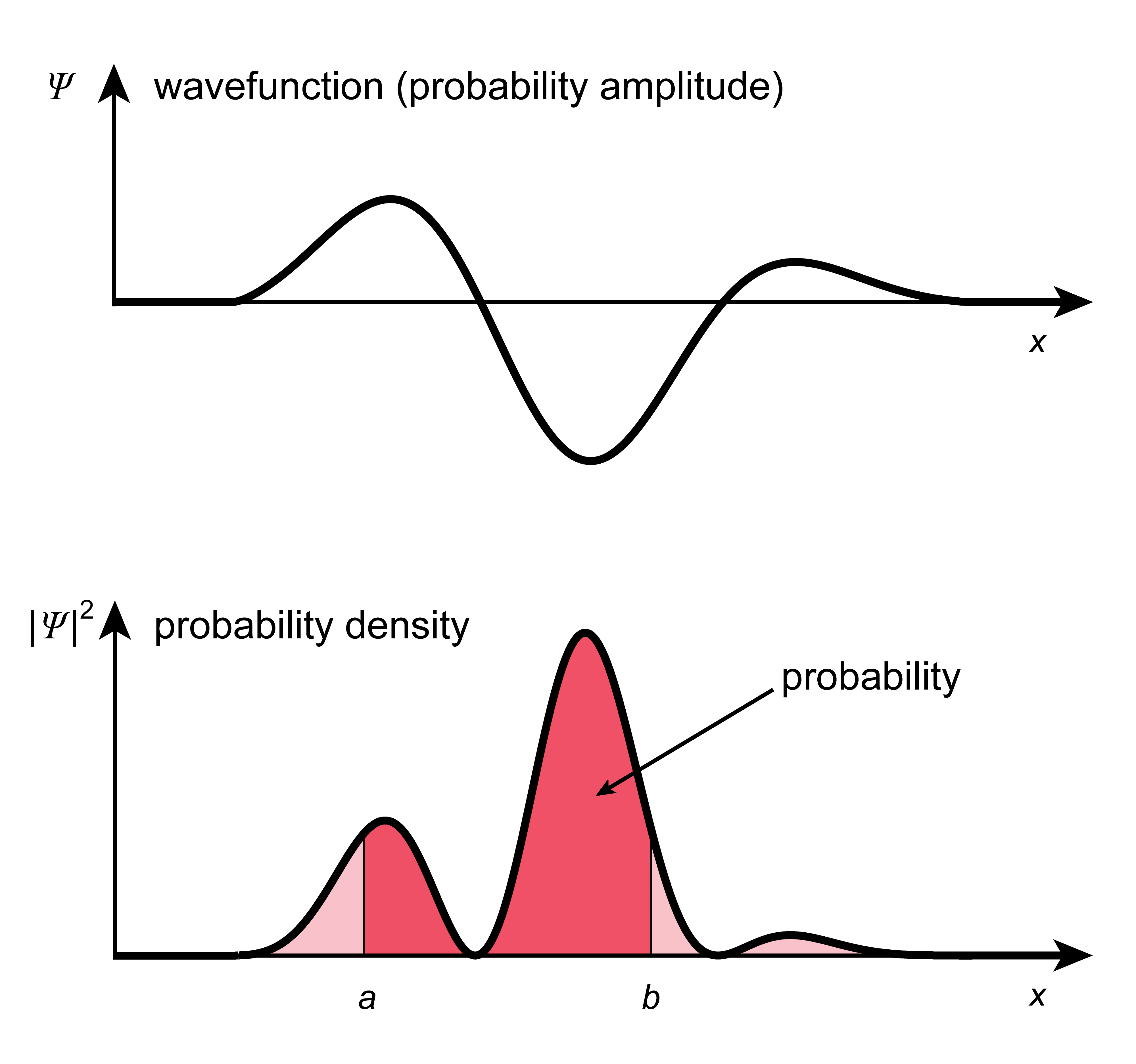
_images/theory_wavefunction.png — Figure 2.2 Wavefunction \(\psi(x)\), probability density \(|\psi(x)|^2\), and probability \(\int_a^b|\psi(x)|^2\mathrm{d}x\).

Note

Delocalization: If the probability density function \(|\psi(x)|^2\) is concentrated strongly in a narrow region, then we say the particle is localized. On the other hand, if \(|\psi(x)|^2\) is spread out and has significant density over a large region, then we say the particle is delocalized.

Since the probability of finding the particle somewhere in space must be 100% (we are certain it is somewhere), the corresponding integral must be equal to 1:

(2.5)\[\int_{\mathrm{all}\,\,x}\!\psi^*\psi\,\mathrm{d}x = \langle\psi|\psi\rangle = 1\]

A wavefunction that satisfies this is said to be normalized.

The expression with angled brackets is an abbreviated notation for the integral over all positions and is called Dirac bra-ket notation. The angled brackets indicate integration over the full range of all coordinates. The function before the vertical bar is understood to be complex conjugated in the integral. The Dirac notation is quite useful, as it shortens many expressions.

In order to be a physically valid wavefunction, a mathematical function has to satisfy several criteria:

A wavefunction has to be single-valued. This is because its norm-square represents a probability density, and there must be a unique probability density for each position.
A wavefunction must be square integrable. This is because a wavefunction must be normalizable, and the normalization integral must exist and must give a finite value. This generally means that a wavefunction must be finite everywhere and must approach zero as the position coordinates approach \(\pm\infty\).
A wavefunction must be continuous and smooth (continuous first derivative) - no breaks, no kinks. These are properties that derive from the form of the kinetic-energy operator (see Postulate 2).

The following figure illustrates these criteria.

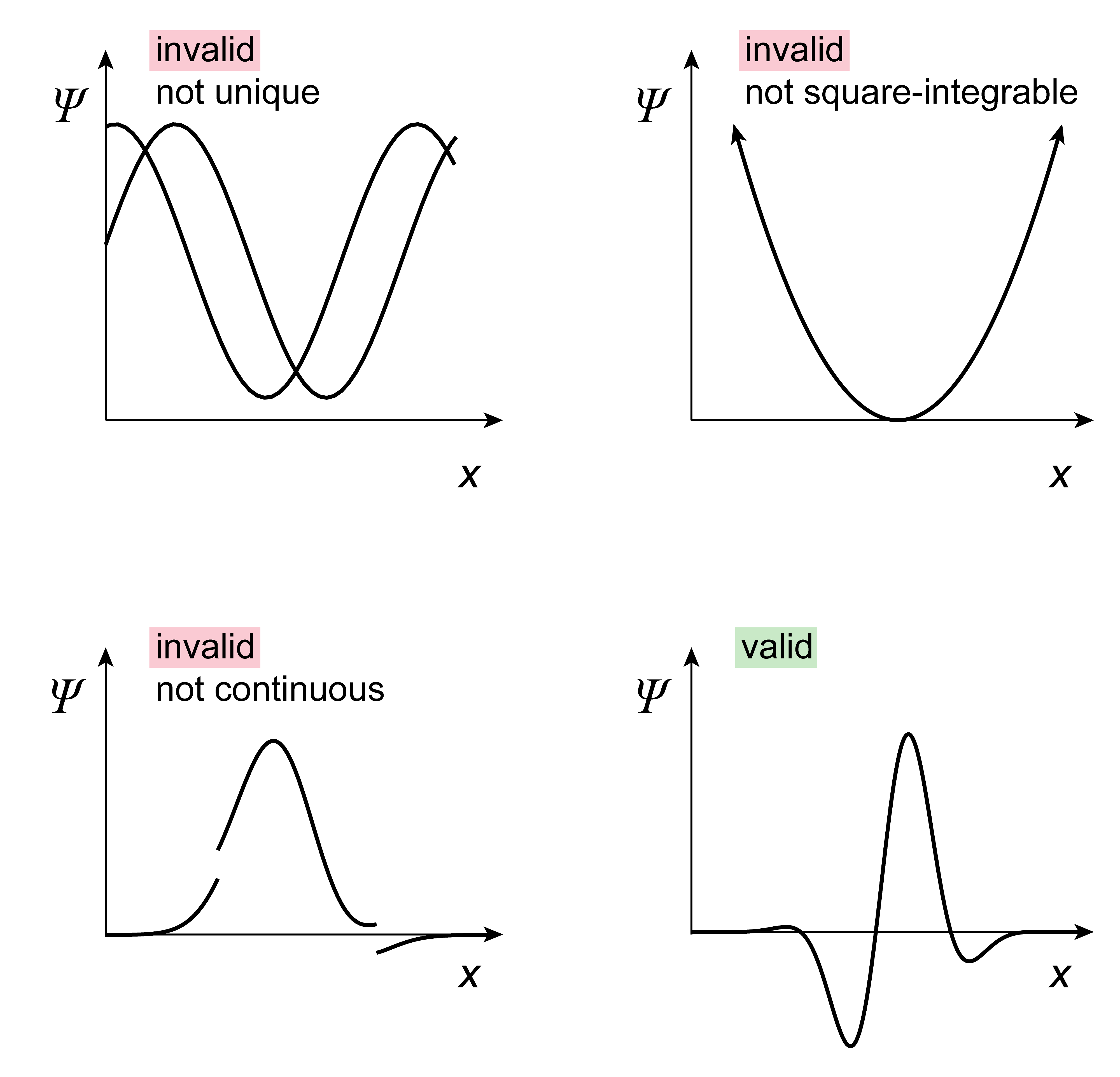
_images/theory_validpsi.png — Figure 2.3 Physically valid and invalid wavefunctions.

Finally, a very important notion is that of orthogonality. Two functions \(\psi_a\) and \(\psi_b\) are said to be orthogonal if

(2.6)\[\int_{\mathrm{all}\,\,x}\! \psi_a^*\psi_b\mathrm{d}x = \langle\psi_a|\psi_b\rangle = 0\]

Note

Do wavefunctions exist? No. A wavefunction is a mathematical model that represents our (incomplete) knowledge about a quantum system, and not something that exists in the real world. This is analogous to making a distinction between a map (which is a model printed on paper or shown on a screen) and the territory it represents (the reality).

2.2. Operators and observables

Postulate 2 of quantum theory states that each observable is mathematically represented by a linear Hermitian operator.

An observable is a property or dynamic variable of a system that can be measured, at least in principle. Examples of observables are the position or the momentum of a particle, or the total energy of a set of particles.

An operator is a prescription or procedure that maps one function onto another function. Notationally, operators are often indicated by a “hat” (circumflex accent):

(2.7)\[\hat{A}f = g\]

Here, the operator \(\hat{A}\) operates on function \(f\) to yield function \(g\).

Note

A simple example of an operator is the first derivative, \(\hat{A} = \mathrm{d}/\mathrm{d}x\). When operating on the function \(f(x) = x^2\), it maps \(x^2\) onto \(2x\), in operator notation \(\hat{A}f(x) = \hat{A}(x^2) = 2x\).

The quantum operator representing a particular observable is obtained via the following general procedure:

Take the classical-physics expression for the observable.
Leave time (\(t\)) and coordinates (\(x\), \(y\), \(z\)) as they are.
Replace the Cartesian components of the linear momentum (\(p_x\), \(p_y\), \(p_z\)) by the following differential operators:

(2.8)\[p_x\rightarrow \hat{p}_x = -\mathrm{i}\hbar\frac{\partial}{\partial x} \qquad \mathrm{etc.}\]

For example, the classical expression for the kinetic energy of a particle of mass \(m\) moving in three dimensions is

(2.9)\[T = \frac{1}{2}m\left\|\boldsymbol{v}\right\|^2 = \frac{1}{2m}\left\|\boldsymbol{p}\right\|^2 = \frac{1}{2m}\left(p_x^2+p_y^2+p_z^2\right)\]

where the velocity \(\boldsymbol{v}\) and the linear momentum are related by \(\boldsymbol{p} = m\boldsymbol{v}\). Substituting the momentum operators gives the quantum version:

(2.10)\[\hat{T} = \frac{1}{2m}\left(\hat{p}_x^2+\hat{p}_y^2+\hat{p}_z^2\right) = -\frac{\hbar^2}{2m}\left(\frac{\partial^2}{\partial x^2}+\frac{\partial^2}{\partial y^2}+\frac{\partial^2}{\partial z^2}\right) = -\frac{\hbar^2}{2m}\nabla^2\]

\(\nabla^2\) (“nabla squared” or “del squared” or “Laplacian”) is an abbreviation for the sum of second derivatives. If the motion of the particle is restricted to one dimension, the kinetic energy is

(2.11)\[\hat{T} = -\frac{\hbar^2}{2m} \frac{\mathrm{d}^2}{\mathrm{d} x^2}\]

Most operators in quantum theory are either multiplicative or derivatives. Below is a list of important observables for a one-particle system and their corresponding operator representations in quantum theory.

Observable	Operator
position along \(x\), \(y\), \(z\)	\(\hat{x} = x\cdot\), etc.
position vector	\(\hat{\boldsymbol{r}} = (\hat{x},\hat{y},\hat{z})\)
momentum along \(x\), \(y\), \(z\)	\(\hat{p}_x = -\mathrm{i}\hbar\frac{\partial}{\partial x}\), etc.
momentum vector	\(\hat{\boldsymbol{p}} = (\hat{p}_x,\hat{p}_y,\hat{p}_z)\)
velocity along \(x\), \(y\), \(z\)	\(\hat{v}_x = \hat{p}_x/m = -\mathrm{i}\frac{\hbar}{m}\frac{\partial}{\partial x}\), etc.
angular momentum vector	\(\hat{\boldsymbol{l}} = \hat{\boldsymbol{r}}\times\hat{\boldsymbol{p}}\)
angular momentum along along \(z\)	\(\hat{l}_x = \hat{y}\hat{p}_x - \hat{z}\hat{p}_y\)
potential energy	\(\hat{V} = V(x,y,z)\cdot\)
kinetic energy	\(\hat{T} = -\frac{\hbar^2}{2m}\nabla^2\)
total energy	\(\hat{H} = \hat{T} + \hat{V}\)

The most important operator is the operator representing the total energy. It has a special name - it is called the Hamiltonian operator or simply Hamiltonian and indicated by \(\hat{H}\). It is the sum of the kinetic energy (\(\hat{T}\)) and the potential energy (\(\hat{V}\)). For a single particle of mass \(m\) moving in one dimension, this is

(2.12)\[\hat{H} = \hat{T} + \hat{V} = \frac{\hat{p}^2}{2m} + \hat{V} = -\frac{\hbar^2}{2m}\frac{\mathrm{d}^2}{\mathrm{d}x^2} + V(x)\cdot\]

The Hamiltonian is named after a similar quantity used in classical mechanics. It is of central importance in quantum theory, since it is involved in the Schrödinger equation (see postulate 5 below).

As given by Postulate 2, all operators are linear and Hermitian. An operator \(\hat{A}\) is linear if it satisfies \(\hat{A}(f+g) = \hat{A}f + \hat{A}g\) and \(\hat{A}(cf) = c\hat{A}f\) for any functions \(f\) and \(g\) and any complex scalar \(c\). Examples of linear operators include multiplicative operators (\(x\cdot\)) and derivate operators (\(\mathrm{d}/\mathrm{d}x\)). Examples of non-linear operators include the square root (\(\sqrt{\cdot}\)) or the logarithm \(\mathrm{log}(\cdot)\). Quantum theory uses only linear operators.

A linear operator is called Hermitian if it satisfies

(2.13)\[\int \psi_a^* (\hat{A}\psi_b)\mathrm{d}x = \int (\hat{A}\psi_a)^* \psi_b\mathrm{d}x = \left( \int \psi_b^* (\hat{A}\psi_a)\mathrm{d}x \right)^*\]

or \(\langle\psi_a|\hat{A}\psi_b\rangle = \langle\psi_b|\hat{A}\psi_a\rangle^*\) in bra-ket notation. Not all linear operators are Hermitian, but quantum theory utilizes only linear operators that are also Hermitian to represent observables (non-Hermitian operators are sometimes used, but do not represent observables).

Two operators can be applied to a function in sequence. This is written as

(2.14)\[\hat{A}\hat{B}f = \hat{A}(\hat{B}f)\]

This expression is read and processed right-to-left: First, the operator \(\hat{B}\) is applied to \(f\), and then the operator \(\hat{A}\) is applied to the result.

Note

For example, to apply the operator \(\hat{A}\hat{B}\) with \(\hat{A}=\mathrm{d}/\mathrm{d}x\) (first derivative) and \(\hat{B} = x\) (multiplication by \(x\)) to the function \(f(x) = \sin(kx)\), start with applying \(\hat{B}\), and then apply \(\hat{A}\) to the result:

(2.15)\[\hat{A}\hat{B}f(x) = \frac{\mathrm{d}}{\mathrm{d}x}\left(x f(x)\right) = \frac{\mathrm{d}}{\mathrm{d}x}\left(x \sin(k x)\right) = \sin(k x) + x k \cos(kx)\]

On the other hand, to apply \(\hat{B}\hat{A}\), start with \(\hat{A}\) and then apply \(\hat{B}\) to the result:

(2.16)\[\hat{B}\hat{A}f(x) = x \frac{\mathrm{d}}{\mathrm{d}x}\left( f(x)\right) = x k \cos(kx)\]

Another important concept in quantum theory is the commutator of two operators \(\hat{A}\) and \(\hat{B}\). The commutator is the difference between the two different ways of applying the two operators, \(\hat{A}\hat{B}\) and \(\hat{B}\hat{A}\). The commutator is indicated by square brackets and is defined as

(2.17)\[[\hat{A},\hat{B}] = \hat{A}\hat{B}-\hat{B}\hat{A}\]

If the commutator of two operators is zero, the two operators are said to commute, and it does not matter in which order they are applied to a function.

Note

Commuting and non-commuting operators. Take the two operators \(\hat{A}=\mathrm{d}/\mathrm{d}x\) and \(\hat{B}=x\). To calculate their commutator \([\hat{A},\hat{B}]\), it’s best to apply it to a generic function \(f\):

(2.18)\[\begin{split}\begin{align} [\hat{A},\hat{B}]f &= \left( \hat{A}\hat{B}-\hat{B}\hat{A} \right)f = \hat{A}\hat{B}f-\hat{B}\hat{A}f \\ &= \frac{\mathrm{d}}{\mathrm{d}x} \left(x f\right) - x \frac{\mathrm{d}f}{\mathrm{d}x} = f \end{align}\end{split}\]

The commutator is \([\mathrm{d}/\mathrm{d}x,x] = 1\) and is non-zero. The two operators do not commute. An example of two operators that commute is \(\hat{A}=\mathrm{d}/\mathrm{d}x\) and \(\hat{B}=y\).

2.3. Eigenvalues and eigenfunctions

Quantum theory is not able to predict with certainty the outcome of a single measurement on a single molecule. Rather, it predicts the possible outcomes and their associated probabilities. Postulate 3 states that the only possible outcomes of a measurement of an observable on a single quantum system are the eigenvalues of the corresponding operator.

The eigenvalues of an operator \(\hat{A}\) are obtained from the following eigenvalue equation:

(2.19)\[\hat A\psi_k = a_k\psi_k\]

Any function \(\psi_k\) that satisfies this equation is said to be an eigenfunction of the operator \(\hat{A}\), and \(a_k\) is called the eigenvalue of \(\hat{A}\) associated with \(\psi_k\). “Eigen” is German for “inherent”, so the eigenvalues and eigenfunctions of an operator are the inherent values and functions associated with that operator. There are typically infinitely many different \(\psi_k\) with associated eigenvalues. According to the postulate, the possible outcomes are given by the set of all \(a_k\). Which one among them is obtained in a particular experiment is not predicted by quantum theory.

Note

Example: For the operator \(\mathrm{d}^2/\mathrm{d}x^2\), the functions \(\psi = \sin(k x)\) are eigenfunctions with eigenvalues \(-k^2\), since

(2.20)\[\frac{\mathrm{d}^2}{\mathrm{d}x^2}\sin(k x) = k \frac{\mathrm{d}}{\mathrm{d}x}\cos(k x) = -k^2 \sin(k x)\]

The second part of Postulate 3 states that when the outcome \(a_k\) is observed, the wavefunction changes from \(\psi\) to \(\psi_k\).

Note

The change of \(\psi\) to \(\psi_k\) upon observation of outcome \(a_k\) is often called wavefunction collapse and interpreted as something real and mysterious. However, recall that a wavefunction is just a mathematical representation of our (incomplete) knowledge about the state of the system, so that it is not surprising that the arrival of new information (an observed measurement value \(a_k\)) necessarily changes this knowledge, and therefore the wavefunction. We take the new wavefunction, and the old one becomes obsolete.

In the context of eigenvalues and eigenfunctions, we need to introduce two important properties of Hermitian operators: (1) Their eigenvalues are real-valued. (2) Their eigenfunctions with different eigenvalues are orthogonal. (You can find proofs of these properties in more advanced textbooks on quantum theory.)

The eigenfunctions of a Hermitian operator form a complete orthogonal set in the sense that any reasonably behaved function \(\psi\) can be written as a linear combination of these eigenfunctions.

(2.21)\[\psi(x) = \sum_{k=1}^{\infty} c_k\psi_k(x)\]

The coefficients \(c_k\) are called expansion coefficients or linear-combination coefficients and can be calculated via

(2.22)\[c_k = \langle\psi_k|\psi\rangle = \int_{-\infty}^\infty \psi_k^*(x)\psi(x) \mathrm{d}x\]

The quantity \(\langle\psi_k|\psi\rangle\) is said to be the projection of \(\psi\) onto \(\psi_k\). If the functions in the orthogonal set are normalized, the set is said to be orthonormal:

(2.23)\[\langle\psi_a|\psi_b\rangle = \delta_{ab}\]

where \(\delta_{ab}\) is the Kronecker delta, equal to zero if \(a\neq b\) and equal to 1 if \(a=b\).

2.4. Expectation values

The second important prediction of quantum theory about the outcomes of measurements is probabilistic in nature: For a given observable, it is possible to predict the average of the outcomes, when averaged over a large set of \(N\) independent experiments on \(N\) identical and identically prepared systems, in the limit of \(N\) becoming infinitely large. This predicted long-run average is also called the expectation value and indicated by angled brackets. According to postulate 4, the expectation value of an observable \(A\) is

(2.24)\[\langle A\rangle = \langle\psi|\hat{A}|\psi\rangle = \int\psi^*\hat{A}\psi\,\mathrm{d}x\]

if \(\psi\) is normalized, or \(\langle A\rangle = \langle\psi|\hat{A}|\psi\rangle/\langle\psi|\psi\rangle\) if \(\psi\) is not normalized.

Note

The expectation value itself is typically different from all the possible outcomes. For example, assume measuring the energy of a quantum system has two possible outcomes, say 5.00 eV with 50% probability and 8.00 eV with 50% probability, the expectation value (predicted long-term average over many measurements) is 6.50 eV. However, 6.50 eV is not a possible outcome - the only possible ones are 5.00 eV and 8.00 eV.

The following figure illustrates the connection between possible outcomes, actual outcomes of individual measurements, and the expectation value.

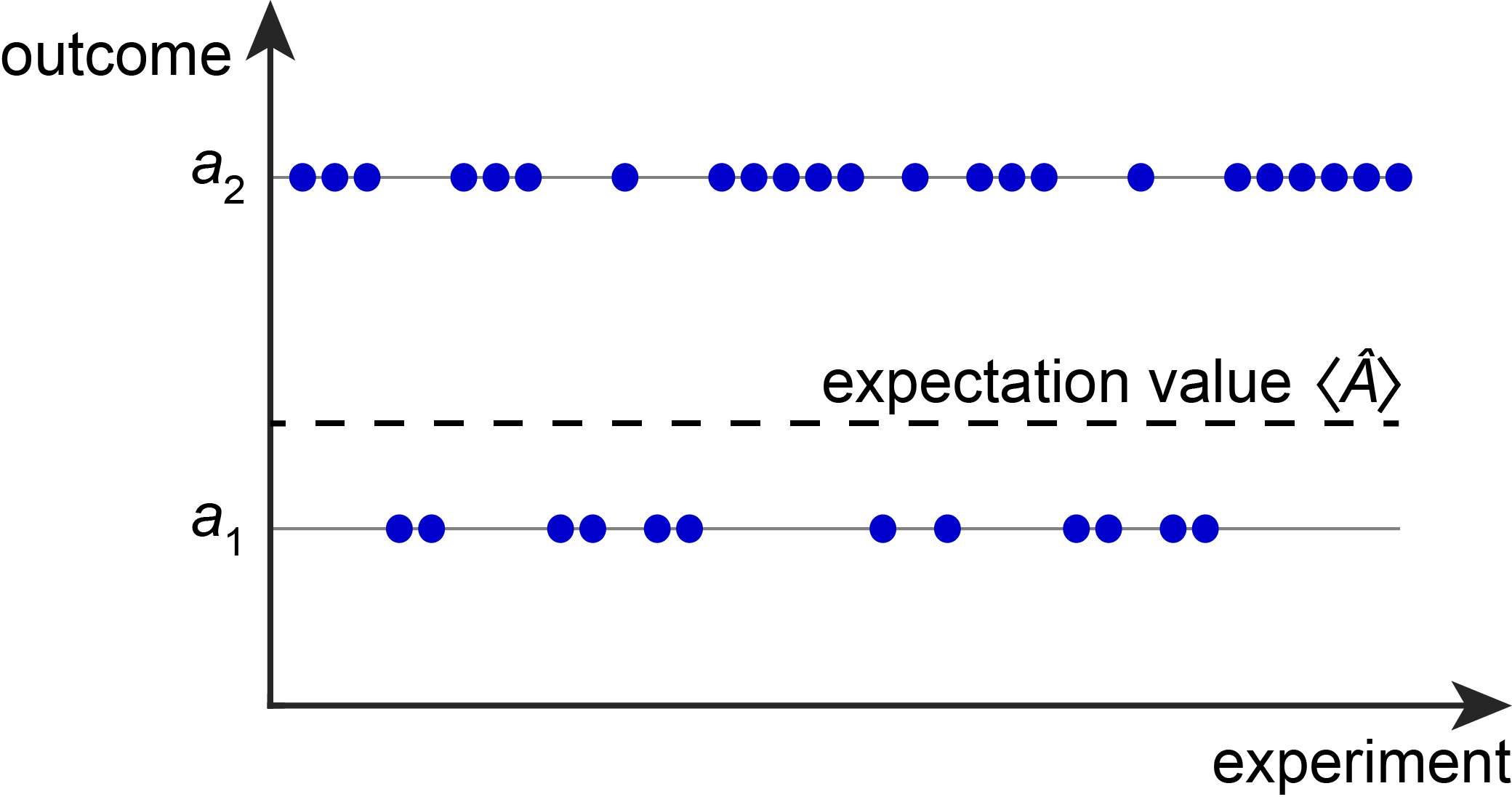
_images/theory_expectation.png — Figure 2.4 A series of measurements of property \(A\) on many identical systems will yield a series of outcomes, each of them one of the eigenvalues of \(\hat{A}\). Their average will converge to the expectation value.

From this postulate, it is also possible to derive the value for the probabilities that outcome \(a_k\) is observed when \(A\) is measured on a system in state \(\psi\). This probability is

(2.25)\[\mathrm{Prob}(a=a_k|\psi) = |\langle\psi_k|\psi\rangle|^2\]

which is the square of the projection of \(\psi\) onto \(\psi_k\).

Note

Here is an example. Take the wavefunction \(\psi = c_1\psi_1 + c_2\psi_2\), where the \(\psi_k\) are eigenfunctions of the energy (i.e. \(\hat{H}\psi_1=E_1\psi_1\) and \(\hat{H}\psi_2=E_2\psi_2\)). The expectation value for the energy is

(2.26)\[\langle E\rangle = \langle\psi|\hat{H}|\psi\rangle = \langle c_1\psi_1 + c_2\psi_2|\hat{H}| c_1\psi_1 + c_2\psi_2\rangle\]

which expands to

(2.27)\[= |c_1|^2 \langle \psi_1|\hat{H}|\psi_1\rangle + c_2^*c_1 \langle\psi_2|\hat{H}|\psi_1\rangle + c_1^*c_2 \langle\psi_1|\hat{H}|\psi_2\rangle + |c_2|^2 \langle \psi_2|\hat{H}|\psi_2\rangle\]

Since the wavefunctions \(\psi_k\) are orthonormal, the integrals in the second and third term are zero, and the integrals of the first and the last term are one. We therefore obtain

(2.29)\[\langle E\rangle = |c_1|^2 E_1 + |c_2|^2 E_2\]

The factors \(|c_1|^2\) and \(|c_2|^2\) are the probabilities for obtaining \(E_1\) and \(E_2\) in a measurement, respectively. These can be obtained by projection, for example

(2.30)\[|\langle|\psi_1|\psi\rangle|^2 = |\langle|\psi_1|c_1\psi_1+c_2\psi_2\rangle|^2 = |c_1\langle\psi_1|\psi_1\rangle+c_2\langle\psi_1|\psi_2\rangle|^2 = |c_1|^2\]

2.5. Uncertainty relation

From the wavefunction \(\psi\) describing a particular state, we can calculate more than just the expectation value of an observable \(A\). For example, we can obtain the expected root-mean-square (or standard) deviation \(\Delta A\) of the observable \(A\) via

(2.31)\[\Delta A = \sqrt{\langle A^2\rangle - \langle A\rangle^2}\]

with \(\langle A\rangle = \langle\psi|\hat{A}|\psi\rangle\) and \(\langle A^2\rangle = \langle\psi|\hat{A}^2|\psi\rangle\). This is a measure of the spread of the measurement outcomes when \(A\) is measured. The spread is positive or zero, but never negative.

Now it can be shown that the product of two root-mean-square deviations of two observables satisfies the following very general relation (see derivation):

(2.32)\[\Delta A\cdot \Delta B \ge \frac{1}{2}\left|\langle[\hat{A},\hat{B}]\rangle\right|\]

The right-hand side contains the commutator of the two operators, \([\hat{A},\hat{B}] = \hat{A}\hat{B}-\hat{B}\hat{A}\). If \(\hat{A}\) and \(\hat{B}\) commute, then the right-hand side is zero, and one or both of the standard deviations can be zero. However, if the operators do not commute, then the right-hand side provides a positive lower limit - meaning that neither standard deviation is zero.

Applied to position and momentum along the same dimension (\(\hat{A} = \hat{x}\) and \(\hat{B} = \hat{p}_x\)), the commutator is \([\hat{x},\hat{p}_x] = \mathrm{i}\hbar\). With this, we get the famous Heisenberg uncertainty relation:

(2.33)\[\Delta x \cdot\Delta {p_x}\ge\frac{1}{2}\hbar\]

\(\Delta x\) describes the predicted spread in position measurements, and \(\Delta p_x\) the predicted spread of momentum measurements:

(2.34)\[\Delta x = \sqrt{\langle x^2\rangle - \langle x\rangle^2} \qquad \Delta p_x = \sqrt{\langle p_x^2\rangle - \langle p_x\rangle^2}\]

The uncertainty relation indicates that there is no state (described by any wavefunction) where position and momentum are both precisely predictable. It expresses a fundamental limit on how well quantum theory can simultaneously predict position and momentum.

Note

Here is one way to parse the meaning of the Heisenberg uncertainty relation. Take 2000 identical copies of a quantum system (for example, a particle in a box), all prepared to be in the same state. On 1000 of them, measure the position, \(x\), and calculate the standard deviation of these 1000 measurements, \(\Delta x\). On the other 1000, measure the momentum \(p_x\) and calculate the standard deviation of these 1000 measurements, \(\Delta p\). For this situation, the Heisenberg uncertainty princple predicts that the product of the two standard deviations is never smaller \(\hbar/2\).

There exists an uncertainty relation involving the energy and the lifetime of excited states. This, however, has a different origin, since time is not an operator in quantum theory, but a parameter.

2.6. Schrödinger equation

The final postulate concerns the prediction of how a state of a quantum system changes over time. It states that the time evolution of a wavefunction is goverened by the time-dependent Schrödinger equation, for a single particle in one dimension given by

(2.35)\[\hat{H}\varPsi(x,t) = \mathrm{i}\hbar\frac{\partial\varPsi(x,t)}{\partial t}\]

This equation is the central equation of quantum theory.

In this book, we limit ourselves to stationary states, i.e. states whose properties are time independent. The wavefunctions of stationary states can be written as a single product of a spatial part and a temporal part: \(\varPsi(x,t) = \psi(x)\cdot f(t)\). That these wavefunctions correctly describe stationary states can be seen as follows:

(2.36)\[\langle\varPsi|\hat{A}|\varPsi\rangle = \langle\psi f|\hat{A}|\psi f\rangle = |f|^2 \langle\psi|\hat{A}|\psi\rangle = \langle\psi|\hat{A}|\psi\rangle\]

We see that they lead to time-independent expectation values, for any operator \(\hat{A}\).

Inserting \(\varPsi = \psi f\) into the Schrödinger equation, and assuming that the Hamiltonian is time-independent, an equation for the spatial part alone is obtained:

(2.37)\[\hat{H}\psi(x) = E\cdot\psi(x)\]

(see derivation). This is called the time-independent Schrödinger equation and is just the eigenvalue equation for the total energy. The time-dependent part is \(f(t) = \mathrm{exp}(-\mathrm{i}Et/\hbar)\), a complex exponential of magnitude 1.

Note

Any normalized function is a physically valid wavefunction. It does not necessarily have to satisfy the time-independent Schrödinger equation. Those functions that do represent stationary states, i.e. states whose measurable properties (observables) do not change over time. All other wavefunctions still satisfy the time-dependent Schrödinger equation and describe non-stationary states.

In the remainder of this book, we will focus on solving the time-independent Schrödinger equation (eigenvalue equation for the total energy) for many different systems. We start with simple toy models and then use it to describe molecular vibrations and rotations, as well as the internal structure of atoms and molecules.