S=2 simulations

[Emilien]

Hello,
I try to simulate S=2 spectra from Fe II proteins, in parallel mode.
First of all I'd like to reproduce a simulation found in the litterature (Hendrich, BiophysJ 1989), Fig 5.a.

Hendrich1989.jpg (123.34 KiB) Viewed 6730 times

Here is the code I wrote:

Code: Select all

Sys.S=2;
Sys.g=[2 2.06 2.14];
D=-8;%K 
E=-2.05;%K
Sys.D=[D E]*0.7*29979.2458;%in cm-1 in MHz
Sys.DStrain=[0 0.60]*0.7*29979.2458;%K in cm-1 in MHz
 
Exp.Range=[0 300];%mT
Exp.mwFreq=9.1;%GHz;
Exp.Temperature=4;%K
Exp.Mode='parallel';

[x,y]=pepper(Sys,Exp);
plot(x,y)

Unfortunately, no resonance is found at 9.1GHz. E has to be increase to -1K to see something...
I can not understand why my easyspin simulation can not reproduce Hendrich's one and where I am wrong...
I would appreciate some help!
Thanks!

[thanasis]

I corroborate.

From what I see your model correctly reproduces the parameters in the legend.

Just to note that D = -8 K means D = -166.68 GHz ( = -8 * 0.695 * 2.9979e+04 / 1e3) as you correctly convert, and the two lowest-lying sublevels are 32.1 GHz (1.1 cm^-1) apart. Little wonder nothing shows up at 9.1 GHz.

I added the following to your code to do Zeeman plots.

...
figure(1)
plot(x,y)

figure(2)
Par.Units = 'cm^-1';
% Par.Units = 'GHz';
Par.PlotThreshold = 0;
Ori='z'; FieldRange=Exp.Range;
Freq = Exp.mwFreq; % GHz
Par.nPoints=1e3;
Par.Mode = Exp.Mode;
Par.Temperature = Exp.Temperature;
levelsplot(Sys,Ori,x,Freq,Par)

[Matt Krzyaniak]

If you crank up the orientations(Opt.nKnots or Opt.GridSize) and shift to higher field range you can see some structure with these parameters around 5500 mT...

They could be catching a low field tail from the higher field structure, or the paper(and their simulation) had slightly wrong values...

[Emilien]

I have an experimental spectra that looks like the one in the figure 5.
Unfortunately easyspin seems not to be able to simulate this spectra... whatever the parameters are...
Moreover, I found some simulated spectra in the litterature. I can not imagine that they all are wrong...

[Matt Krzyaniak]

Well consider:

Code: Select all

clear
Sys.S=2;
Sys.g=[2 2.06 2.14];
D=-8;%K 
E=-2.05;%K
conv = 1e-6*boltzm/planck; % MHz/K
Sys.D=[D E]*conv;
%Sys.DStrain=[0 0.60]*0.7*29979.2458;%K in cm-1 in MHz

% Zerofield energies as per ES 
ham = sham(Sys,[0 0 0]);
[V,E]= eig(ham); 
diag(E)/1000 % GHz

% Zerofield levels as defined pg491 of Hendrich, BiophysJ 1989
[-2*sqrt(Sys.D(1)^2+3*Sys.D(2)^2);
2*Sys.D(1);
-Sys.D(1)+3*Sys.D(2);
-Sys.D(1)-3*Sys.D(2);
2*sqrt(Sys.D(1)^2+3*Sys.D(2)^2);]/1000

Both of which agree to give in GHz:

Code: Select all

ans =

 -364.7480
 -333.3859
   38.5477
  294.8382
  364.7480

And as you turn on the magnetic field, the lower two levels are only going to separate further. The paper suggests it is these two levels which give rise to the transition observed in the spectrum. Which means that the observed transition must be from a strained component, or a distribution in E. Given that sigmaE = 0.6 K I would guess that the simulation really only comes from the edge of the distribution. So the only thing that I could point to is difference in how the strain in modeled in that paper vs ES.

The upper two will get closer, but with an initial splitting of 74 GHz splitting, it will only show a 9 GHz resonance at fairly high fields.

[Emilien]

The strain is modeled by a gaussian distribution both in ES and in the paper. The only difference is how is characterized this gaussian distribution. FWHM is used in ES. Standard deviation is used in the paper (FWHM=2.sigma.(2.ln(2))^0.5=2.3548.sigma).
Then I replace the corresponding line in the first code with

Code: Select all

Sys.DStrain=[0 2.3548*0.60]*0.7*29979.2458;%K in cm-1 in MHz

And no resonance field is found at 9.1GHz...

You are totally right when saying

the simulation really only comes from the edge of the distribution

Let's determine the E values giving resonance(s) with constant D and 0=<E/D<=1/3, and see if these values are included in the E-distribution

Code: Select all

Sys.S=2;
Sys.g=[2 2.06 2.14];
D=-8;%K 
E=linspace(-8/3,0,100); % 0<=E/D<=1/3
 
Exp.Range=[0 300];%mT
Exp.mwFreq=9.1;%GHz;
Exp.Temperature=4;%K
Exp.Mode='parallel';

Opt.Threshold=0;
Opt.Sparse=0;

%%% E values leading to resonance field
for k=1:numel(E)
    Sys.D=[D E(k)]*0.7*29979.2458;%in cm-1 in MHz
    data{k,1}=resfields(Sys,Exp,Opt); %resonance position(s)
end

%%%gaussian distribution of E and intersection with E values giving resonance
probaE=gaussian(E,-2.05,0.6*2.3548);
index_res=~cellfun(@isempty,data(:,1));%index where resonance is found
plot(E,probaE); % E dsitribution
hold on
area(E(index_res),probaE(index_res))
xlabel('E (K)')
title('E distribution')

The execution of this code gives:

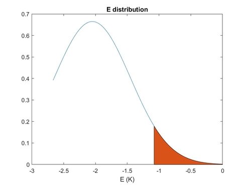
E_distribution_reduced.jpg (21.65 KiB) Viewed 6644 times

The colored edge of the distribution represents the E values with resonance.
Why ES and especially pepper does not take this edge of the distribution into account, even if no resonance arises from the central value of the E distribution?

Thanks for your help!

[Matt Krzyaniak]

I needed to brush up on exactly how ES was treating this.
Within resfields, ES is not explicitly calculating a distribution of D and E value when using Dstrain but rather an anisotropic broadening factor. So when the central feature, as is the case in your simulation, has no resonance there is nothing to broaden. In fact, the line broadening page in the documentation does provide a work around, which you've nearly reproduced in your above script.

Code: Select all

clear
Sys.S=2;
Sys.g=[2 2.06 2.14];
Sys.lwpp = 5;
D=-8;%K 
E=linspace(-8/3,0,100); % 0<=E/D<=1/3
probaE=gaussian(E,-2.05,0.6*2.3548);

Exp.Range=[0 300];%mT
Exp.mwFreq=9.1;%GHz;
Exp.Temperature=4;%K
Exp.Mode='parallel';

Opt.Threshold=0;
Opt.Sparse=0;

%%% E values leading to resonance field
spec = 0;

index_res = logical(zeros(size(E)));
for k=1:numel(E)
    Sys.D=[D E(k)]*0.7*29979.2458;%in cm-1 in MHz
    [B,spec_] = pepper(Sys,Exp,Opt);
   spec = spec + probaE(k)*spec_; %resonance position(s)
   index_res(k) = any(spec_);
end

subplot(2,1,1); plot(E,probaE); axis tight
hold on
area(E(index_res),probaE(index_res))
xlabel('E (K)')
hold off
subplot(2,1,2); plot(B,spec); axis tight

Choppiness is observed due to not enough sampled orientations or not enough line broadening.

[Stefan Stoll]

Indeed, this is one of these situations where ES's DStrain approach (take the resonance field, and calculate the broadening using its derivatives with respect to D and E) is not applicable, and an explicit loop over a spin Hamiltonian parameter distribution is needed.

There is an example for this in the documentation here, but I think we should add a note about this directly to the section on DStrain.